UAV Method Based on Multispectral Imaging for Field Phenotyping

Editors: Ndjido A. Kane, Daniel Foncéka, and Timothy J. Dalton

7 UAV Method Based on Multispectral Imaging for Field Phenotyping

Modou Mbaye, ISRA/CERAAS, Senegal

Adama Ndour, ICRISAT, Mali

Boubacar Gano, Cheikh Anta Diop University of Dakar, Senegal & ISRA/CERAAS, Senegal

Joseph Dembele, Cheikh Anta DIOP University of Dakar, Senegal & ISRA/CERAAS, Senegal

Delphine Luquet, CIRAD, France

Gregory Beurrier, CIRAD, France

Alain Audebert, CIRAD, France & ISRA/CERAAS, Senegal

Abstract

In many countries, particularly in West Africa, there is a strong social demand for increased cereal production. Responding to this demand involves the improvement of cereal varieties. Modern varietal breeding programs in the sub-region need to establish the relationship between plant genotype and phenotype to select high-yielding stress-tolerant plants and to enhance agricultural production. However, in most cases, accurate phenotyping of large mapping populations is a limiting factor. The Regional Study Centre for the Improvement of Drought Adaptation (CERAAS) has developed a robust drone-based data collection and spatial modelling process to better measure cereal crops’ traits for the benefit of plant breeding programs. Herein, we report an unmanned aerial vehicle (UAV) driven crop characteristics analysis throughout the crop cycle. We present a fully automatic pipeline based on a multispectral imaging system for the indirect measurement of agronomic and phenological characters of crops in agricultural field trials. The pipeline is made up of different stages including image acquisition, georeferencing, generation of orthoimages, creation of masks to delimit individual plots, and calculation of proxies. The incorporation of the UAV into agricultural field experiments has the potential to fast-track the genetic improvement of adaptation to drought.

Keywords: UAV, multispectral, field phenotyping, sorghum

Introduction

If the world’s population and food demand continue to grow, food production will need to increase 60% by 2050. It is urgent to develop new strategies to feed future generations. Over the last few decades, many breeding programs have focused on the improvement of major traits for crop varieties such as yield, disease resistance, and resistance to other environmental constraints (Cuenca et al., 2013). Nowadays, breeding methodologies employ innovative digital tools such as artificial intelligence, bioinformatics, genomics, and statistical advances to enable the speedy creation of cultivars (Vardi et al., 2008). A fundamental condition to new breeding methods such as genomic selection is the development of a training population with an exceedingly high genetic diversity (Aleza et al., 2012). Therefore, carrying out large-scale plant phenotyping experiments is critical; the fast and precise collection of phenotypic data is especially important to explore the association between genotypic and phenotypic information.

In Africa, sorghum is the second major staple cereal and constitutes the only viable food for the most food-insecure populations of the world (Hariprasanna & Rakshit, 2016). However, its genetic improvement relies mostly on manual phenotyping. Traditional phenotyping techniques are often expensive, labor-intensive, and time-consuming (Cruz et al., 2017; Luvisi et al., 2016). Using unmanned aerial vehicles (UAV) equipped with sensors has recently been considered as a cost-effective alternative tool for rapid, accurate, non-destructive, and noninvasive high-throughput phenotyping (Pajares, 2015). However, the measurements of plant traits using UAVs are carried out through vegetation indices obtained by image processing. Many studies demonstrated the efficient use of UAV to monitor plant biomass (Lussem et al., 2019), crop health status, nitrogen content, plant water need estimates (Romero et al., 2018), or even to help in the detection of plant diseases (Abdulridha et al., 2018). Unlike satellites, UAVs represent a relatively low-cost method for image acquisition with high resolution and they are increasingly used for agricultural applications. Hunt et al. (2010) established a good correlation between leaf area index (LAI) and normalized difference vegetation index (NDVI) by using UAV multispectral imaging for crop monitoring. Ribera et al. (2018) deployed UAV trichromatic imagery to count the number of leaves in sorghum. Nebiker et al. (2008) reported the successful application of UAV imagery to evaluate grapevine crop health.

The use of high-performance sensors for plant imaging has resulted in the generation of enormous amounts of image data that required processing to extract useful information. Here, we present our full image processing pipeline to store, preprocess, and analyze sorghum UAV images in a holistic way to extract the spectral indices that correlate the most with structural and physiological variables measured. The pipeline provides valuable information about key priority traits for breeding programs, and it can be used as a decision support tool.

UAV Image Data Acquisition

For this study, images were collected with a hexacopter UAV (FeHexaCopterV2, MikroKopter, Germany) at an altitude of 50 m and a constant speed of 4.5 m.s^-1. This UAV can fly by either remote control or autonomously with Global Positioning Systems. The UAV’s support software (MikroKopter tools, MikroKopter, Germany) implements a flight plan, monitors the flight, and allows information such as drone position. An Airphen multispectral camera (Hyphen, France) with 6 spectral bands (blue = 450 nm, green = 532 nm, green-edge = 568 nm; red = 675 nm; red-edge = 730 nm; NIR = 850 nm) combined with a thermal infrared camera (Flir Ltd, USA) was used. In addition, a RGB SONY ILCE-6000 digital camera (Sony, Japan) with a 6000 x 4000-pixel sensor equipped with a lens of 60 mm focal length was used. To reduce the effects of ambient light conditions, we limited data capturing missions to clear and cloudless days.

Both the RGB and the Airphen multispectral cameras acquired images continuously at 1 Hz frequency. The Hexacopter tools were used to design the flight plan so that it covered all the area and ensured 80% of overlapping both across and along the track. We used a 2.5 m² carpet reference panel placed horizontally on the ground at 1.5 times the height of the closest plants, as recommended by Ahmad et al. (2021). Besides, 6 circular panels of 50 cm diameter were placed in the 4 corners of the field as ground control points (GCPs) (Kääb et al., 2014). The exact positions of these GCPs were defined with GPS GNSS (Global Navigation Satellite System) equipment, providing an accuracy of 2 cm.

Regarding phenotyping in RGB, we calculated proxies from the literature such as the Brightness Index, the Soil Color Index, etc. These indices were shown to have a positive correlation with measured traits.

Figure 1

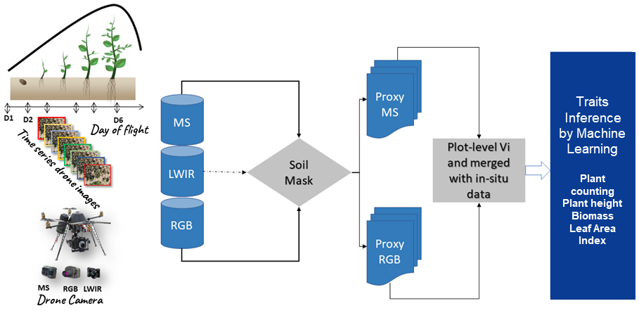
Flow chart showing Field-based UAV Aerial Phenotyping Platform and Methodology Used to Extract the Multispectral Image. Left images show 6-day plant growth & image of drone and camera types (MS, RGB, LWIR). To the right of that are 3 cylinders (MS, RGB, LWIR) point right to diamond shape (Soil Mask). To the right of that are 2 text boxes (Proxy MS & Proxy RGB) pointing right to text box (Plot-level Vi and merges with in-situ data). To the right of that is text box (Traits Inference by Machine Learning & Plant counting Plant height Biomass Leaf Area Index. — Figure 1 – Field-based UAV Aerial Phenotyping Platform and Methodology Used to Extract the Multispectral Image

Note. MS is the multispectral camera, LWIR is the thermal camera, and RGB is the red-green-blue camera. D1 to D6 are the flight dates.

Flight dates are optimized according to the traits of the measured plants. Some traits cannot be measured at certain stages of plant development. For example, if the leaf area is 2 cm, the determination of biomass becomes extremely difficult. Thus, the flight date D1 is used to create a Digital Elevation Model (DEM), which is the field’s reference height (h0). Flight dates D2-D3-D4 are used to measure a plant’s agro-morphological traits, such as biomass, Leaf Area Index (LAI), and plant height. Flight dates D5-D6 are used to assess varieties’ performances at the maturity stage (yield estimation and panicle number). Specific flights are carried out for the characterization of stresses including water, nitrogen, and thermal stresses. The thermal imaging camera is used more during stress characterization to calculate temperature distribution according to cereal varieties.

After the flights, images were uploaded to Agisoft software (Agisoft LLC, St. Petersburg, Russia) to create a geo-referenced multi-layer orthoimage of the flight for each date. A subsample of microplots was designed in both sites and georeferenced using FieldImageR package (Matias et al., 2020). The plot-level reflectance data and vegetation indices were calculated using R (Hijmans & van Etten, 2016). The entire process of spectral index extraction is fully automated, and the outputs are directly obtained in a CSV file.

Workflow of the Image Processing Pipeline

1. Generation of the Orthomosaic Image

All the image datasets collected from every flying date for both cameras were processed separately to generate mosaics of the entire plantation. The RGB imagery was assembled using Agisoft PhotoScan software fully automated scripting API by applying three consecutive phases of superimposed image alignment, field geometry construction, orthoimage, point cloud, and dense surface model (DSM) generation using structure-from-motion algorithms. The final ortho-product is a three-band orthomosaic. Multispectral images were assembled using Agisoft PhotoScan and the multi-band imaging plugin Airphen. The final product was a six-band orthomosaic and a DSM.

2. Radiometric Calibration

Depending on the lighting conditions, sensor configuration, sun position, and measurement angle, the luminance measured by the multispectral sensor occasionally differed from the energy reflected by the crop due to radiometric distortions. To ensure radiometric consistency between the different drone images, radiometric distortions and inconsistencies were accurately processed for subsequent analysis of the images. Radiometric correction consists of converting a digital number of multispectral images into reflectance by absolute or relative calibration (Liang, 2008). In this pipeline, we calibrated the reflectance using a reference surface: the carpet located on the ground at a distance from the plot which was imaged at each flight, and the radiometric calibration tool (Agisoft PhotoScan and the Airphen plugin) which used known reflectance indices of the carpet from laboratory measurements.

3. Geometric Correction

Due to the drone’s speed, altitude, and the angle of sensor view, geometric distortions are possible. As a result, the pixels recorded in the different images might not project onto the same geographical grid due to these distortions. Thus, corrections must be made to increase the spatial coincidence between the images. Firstly, we carried out geometric correction through multiband co-registration to modify and adjust the image coordinate system to decrease geometric distortions and make pixels in different pictures coincide to the similar map grid points. The co-registration process is simply based on internal GPS from raw image metadata. Ortho-rectification was then completed using the GCPs to increase the accuracy of the generated orthomosaic.

4. Extraction of Spectral Vegetation Indices

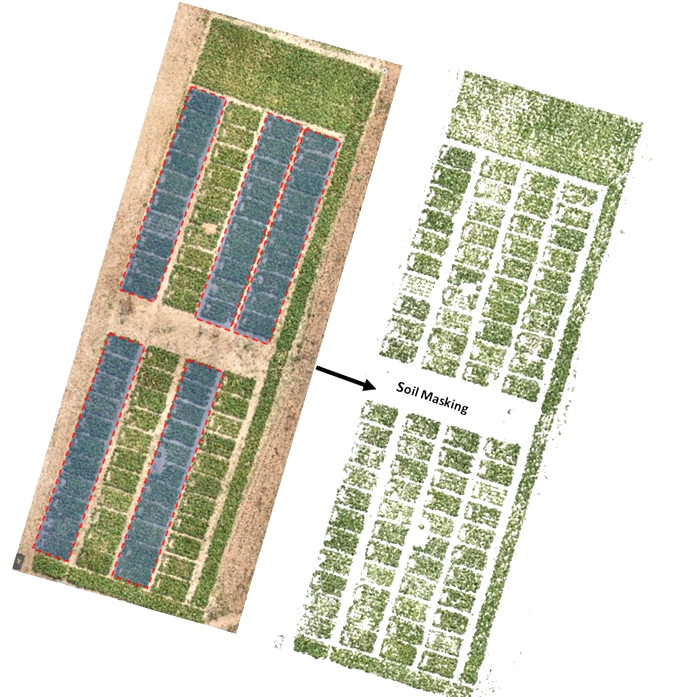
Automated scripts were developed to load RGB and MS orthoimages. Then we used RGB orthomosaic to segment and separate sorghum plants from the soil background by converting mosaics from RGB to HSV colour space and by performing thresholding operations over green pixels to create a sorghum mask. Escadafal’s (1993) modified HUE index was used for effective soil masking of both MS and RGB images. Figure 2 illustrates the output of the soil masking operation. This process is important for reducing bias since the spectral signature of soil mixed with vegetation layers tend to introduce strong outliers.

Figure 2

2 images Obtained After Using the Soil Masking Technique to Extract Both Soil and Vegetation Layers with the Traditional HUE Index Thresholding. Image 1 shows sky view of field plots with 5 areas in gray framed with red dotted lines. An arrow points from this image to Image 2, which is the image without the gray areas, labeled Soil Masking. — Figure 2 – Image Obtained After Using the Soil Masking Technique to Extract Both Soil and Vegetation Layers with the Traditional HUE Index Thresholding

We extracted calibrated reflectance in red, green, and NIR bands using that mask raster. Modified scripts from RSToolbox (Leutner et al., 2017) and FieldImageR (Matias et al., 2020) libraries were used to derive the following well-known spectral indices for crop physiology and biomass monitoring: NDVI, GNDVI, MSAVI2, RVI, CTVI, and NDWI (Table 1). In total, automated extraction of 15 proxies with 7 spectral bands from drone imagery was operated. In addition, the GPS coordinates of each plot were extracted using the QGIS geographic information system software (Menke et al., 2016) and exported as spatial vector data. The extraction of the average values of each vegetation index was performed according to the GPS coordinates extracted on QGIS using the features of the sf and raster packages.

**Table 1**
*Popular Vegetation Indices are Used in Drone Phenotyping with the RGB Camera.*
Vegetation index	Formula
Normalized Ratio Vegetation Index	$NRVI=\frac{R/N -1}{R/N + 1}$
Normalized Difference Water Index	$NDWI=\frac{G-N}{G+N}$
Ratio Vegetation Index	$RVI=\frac{R}{N}$
Green Leaf Index	$GLI=\frac{2R-G-B}{2R+G+B}$
Green Normalized Difference Vegetation Index	$GNDVI=\frac{N-G}{N+G}$
Normalized Difference Vegetation Index	$NDVI=\frac{N-R}{N+R}$
Visible Atmospherically Resistant Index	$VARI=\frac{G-R}{G+R-B}$
Soil Color Index	$SCI=\frac{R-G}{R+G}$
Brightness Index	$BI=\frac{\sqrt{R^{2}+G^{2}+B^{2}}}{3}$
Spectral Slope Saturation Index	$SI=\frac{R-B}{R+B}$
Overall Hue Index	$HUE=\frac{\arctan(2(B-G-R))}{30.5(G-R)}$
Difference Vegetation Index	*$DIV =s(N-R)$**
Corrected Transformed Vegetation Index	$CTVI=\frac{NDVI+0.5}{\sqrt[2]{NDVI+0.5}}$

Figure 3 shows different combinations of orthomosaic bands from the multispectral sensor on field trials of water-stressed and irrigated plots. For each combination, important information can be deduced as parts of the test subjected to water stress or experimental units that are less developed. Figure 3(c) is an overlay of the shapefile of the experimental units with the generated orthomosaic. On each experimental unit, vegetation indices were calculated and further analysis on the spatial modelling on crop characteristics was conducted.

Figure 3

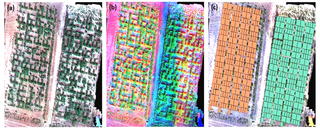
3 images demonstrating Outputs of an RGB Image Showing Spatial Variation Based on Some Vegetation Indices (VIs) on Soil-free Orthomosaic Data. Image (a) shows sky view of 2 identical fields with gray ground and green plants. Image (b) shows sky view of 2 identical fields with various bright colors with more pink on left field and more blue on right field. Image (c) shows sky view of 2 identical fields with orange boxes covering the plots on the left field and green boxes coving the plots on the right field. — Figure 3 – Outputs of an RGB Image Showing Spatial Variation Based on Some Vegetation Indices (VIs) on Soil-free Orthomosaic Data

Note. 3(a) is a True-Color map, while 3(d) is a false-color. 3(c) shows the shapefile generated from each variety.

5. Regression Analysis

Two approaches have been developed in our image processing and analysis pipeline. The first approach uses statistical modelling and machine learning regression to link the agronomic traits to vegetation indices, especially the NDVI. Nevertheless, more than 15 other vegetation indices have been determined including the Soil Color Index (CSI), the Simple Ratio Vegetation Index (SRI), the Green Normalized Difference Vegetation Index (GNDVI), and the Modified Soil Adjusted Vegetation Index (MSAVI). The leaf area index calibrated with data from previous sorghum tests with measurements of NDVI derived from the drone images was estimated according to the statistical model proposed by Gano et al. (2021). An exponential regression law with a coefficient variation of 0.92 was used to estimate the LAI.

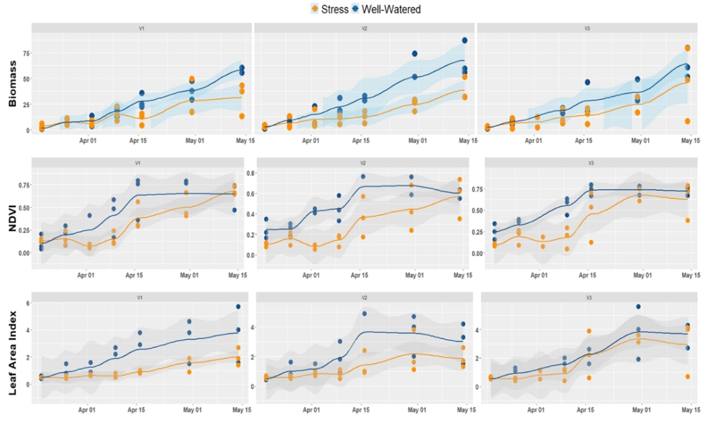
Figure 4 illustrates the spatial-temporal evolution of biomass, NDVI, and LAI of plants grown under water stress and non-stress conditions. This time series plot allowed us to make a rapid survey of how crops are sensitive to stress conditions. It appears from the figure that biomass, as well as LAI, shows a similar trend as the NDVI. This correlation is also noted for other vegetation indices such as GNDVI. Most importantly, water stress decreased the biomass of all the three varieties tested. However, the magnitude of this decrease was not homogeneous across varieties. For example, the variety V3 stands better water stress.

Figure 4

9 line graphs with vertical plot points demonstrating Time Series Analysis of Plant Traits (biomass, NDVI, LAI) in 3 Sorghum Varieties (V1-V3) at Different Dates of Crop Cycle. Graph 1 (Biomass V1) shows gradual increase in Stess (yellow) & Well-Watered (blue) from March 15 to May 15. Graph 2 (Biomass V2) shows gradual increase in Stess (yellow) & Well-Watered (blue) from March 15 to May 15. Graph 3 (Biomass V3) shows gradual increase in Stess (yellow) & Well-Watered (blue) from March 15 to May 15. Graph 4 (NDVI V1) shows gradual increase in Stess (yellow) & Well-Watered (blue) from March 15 to May 15. Graph 5 (NDVI V2) shows gradual increase in Stess (yellow) & Well-Watered (blue) from March 15 to May 15. Graph 6 (NDVI V3) shows gradual increase in Stess (yellow) & Well-Watered (blue) from March 15 to May 15. Graph 7 (Leaf Area Index V1) shows gradual increase in Stess (yellow) & Well-Watered (blue) from March 15 to May 15. Graph 8 (Leaf Area Index V2) shows gradual increase in Stess (yellow) & Well-Watered (blue) from March 15 to May 15. Graph 9 (Leaf Area Index V3) shows gradual increase in Stess (yellow) & Well-Watered (blue) from March 15 to May 15. — Figure 4 – Time Series Analysis of Plant Traits (biomass, NDVI, LAI) in 3 Sorghum Varieties (V1-V3) at Different Dates of Crop Cycle

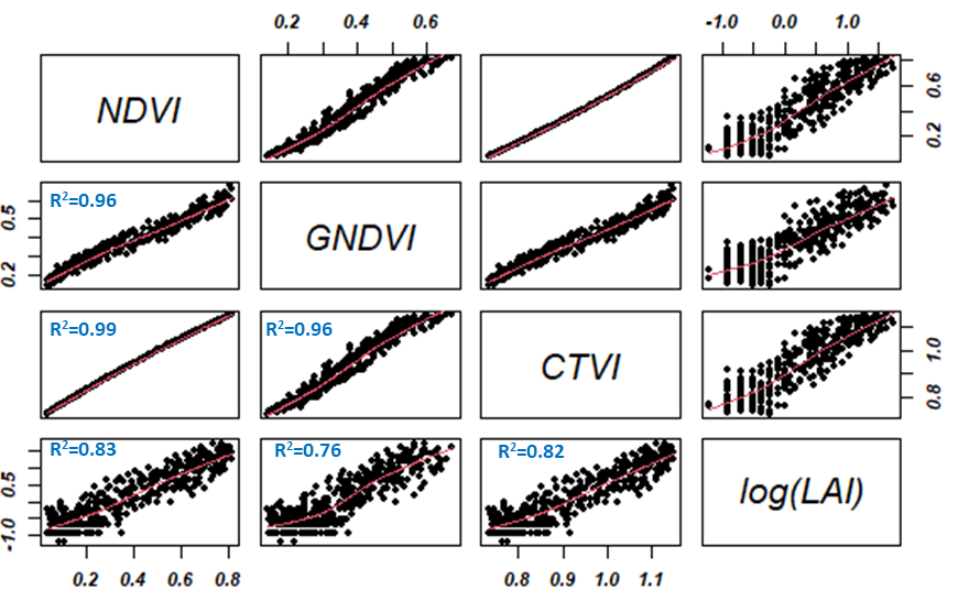
In this report, the regression models developed showed an excellent correlation between LAI and vegetation indices such as NDVI, CTVI, and GNDVI (0.76 < R² < 0.96). Figure 5 illustrates regression analysis and indirect estimation of the LAI. The logarithmic transformation of the LAI shows a linear correlation between the estimated vegetation indices. These indices also have a strong linear dependence of the order of 0.99. From a modeling point of view using one of the indices would give the same result in terms of LAI prediction.

Figure 5

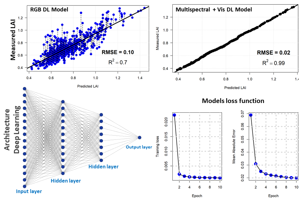
12 scatter plot line charts demonstrating Regression Analysis of Linear Dependency Between Drone Vegetation Index & in Situ LAI showing near linear increase across X axis. — Figure 5 – Regression Analysis of Linear Dependency Between Drone Vegetation Index & in Situ LAI

For the second approach, we used a densely connected neural network to estimate the LAI based on drone vegetation indices and the RGB bands. Our network consisted of four hidden layers with the succession of two drop-out and batch normalization layers. The hidden layers consisted of 128, 64, 128, and 11 units respectively. The drop-out rate was 40% (first layer) and 30% (second layer). We used the Mean Absolute Error as metrics and the Mean Standard Error as loss. For the optimizer, the Gradient Descent with the Root Mean Squared Propagation was used. Deep learning with the above-mentioned vegetation indices showed a better linear relationship with an error of 2% and a coefficient of determination of 0.99. However, deep learning with RGB optical bands produced a 10% error with an R² of 0.7. Figure 6 shows the deep learning regression model for LAI estimation with the deep learning model architecture and the output of the loss function for two different regression models (drone RGB and multispectral).

Figure 6

4 graphs demonstrating A Densely Connected Neural Network for LAI Estimation. Image 1 is scatter plots of the RGB DL Model along linear line showing continued increase from .4 to 1.5 Measured LAI across Predicted LAI X axis. Image 2 is linear plots of the Multispectral + Vix DL Model along linear line showing continued increase from .4 to 1.4 Measured LAI across Predicted LAI X axis. Image 3 shows Architecture Deep Learning with 16 vertical Input layer plot points (left side) connected by lines to 12 vertical Hidden layer plot points connected by lines to 8 vertical Hidden layer plot points connected by lines to 1 Output layer plot point (right side). Image 4 shows 2 graphs for Models of loss function with Training loss dipping from 1 to 2 and then evening out through 10 Epoch on X axis and Mean Absolute Error dipping from 1 to 2 & then evening out through 10 Epoch on X axis. — Figure 6 – A Densely Connected Neural Network for LAI Estimation

The use of statistical regression or deep learning approaches depends on the volume of field data and the experimental data acquisition protocol. However, statistical regression models are more likely to produce bias and prediction errors compared to deep learning models. It is important to note that for large-scale phenotyping, it is much easier to implement statistical models.

Conclusion

In this study, we evaluated the use of multispectral UAV imagery coupled with a fully automated image processing pipeline for the phenotyping of cereal crops. To optimize the computation, we developed 6 proxies from the RGB camera and around 10 other proxies for the multispectral camera. The generation of the shapefile from the experiments is now simplified and allows an easier extraction of the vegetation indices. However, due to the high resolution of the images, the computation time is still long with the processors at our disposal. With this process, we were able to accurately estimate agro-morphological traits using machine learning regression or deep learning architecture.

References

Abdulridha, J., Ampatzidis, Y., Ehsani, R., & de Castro, A. I. (2018). Evaluating the performance of spectral features and multivariate analysis tools to detect laurel wilt disease and nutritional deficiency in avocado. Computers and Electronics in Agriculture, 155, 203–211. https://doi.org/10.1016/j.compag.2018.10.016

Ahmad, A., Ordoñez, J., Cartujo, P., & Martos, V. (2021). Remotely Piloted Aircraft (RPA) in Agriculture: A Pursuit of Sustainability. Agronomy, 11(1), 7. https://doi.org/10.3390/agronomy11010007

Aleza, P., Juárez, J., Hernández, M., Ollitrault, P., & Navarro, L. (2012). Implementation of extensive citrus triploid breeding programs based on 4x x 2x sexual hybridizations. Tree Genetics & Genomes, 8, 1293–1306. https://doi.org/10.1007/s11295-012-0515-6

Cruz, A. C., Luvisi, A., De Bellis, L., & Ampatzidis, Y. (2017). X-FIDO: An effective application for detecting olive quick decline syndrome with deep learning and data fusion. Frontiers in Plant Science, 8, 1741. https://doi.org/10.3389/fpls.2017.01741

Cuenca, J., Aleza, P., Vicent, A., Brunel, D., Ollitrault, P., & Navarro, L. (2013). Genetically based location from triploid populations and gene ontology of a 3.3-Mb genome region linked to Alternaria brown spot resistance in citrus reveal clusters of resistance genes. PloS One, 8(10). https://doi.org/10.1371/journal.pone.0076755

Escadafal, R. (1993). Remote sensing of soil color: Principles and applications. Remote Sensing Reviews, 7(3-4), 261–279. https://doi.org/10.1080/02757259309532181

Gano, B., Dembele, J. S. B., Ndour, A., Luquet, D., Beurier, G., Diouf, D., & Audebert, A. (2021). Using UAV borne, multi-spectral imaging for the field phenotyping of shoot biomass, leaf area index and height of West African sorghum varieties under two contrasted water conditions. Agronomy, 11(5), 850. https://doi.org/10.3390/agronomy11050850

Hariprasanna, K., & Rakshit, S. (2016). Economic importance of sorghum. In S. Rakshit & Y.-H. Wang (Eds.), The sorghum genome (pp. 1–25). Springer International Publishing. https://doi.org/10.1007/978-3-319-47789-3_1

Hijmans, R. J., & van Etten, J. (2016). raster: Geographic data analysis and modeling. R Package Version, 2(8).

Hunt, E. R., Jr., Hively, W. D., Fujikawa, S. J., Linden, D. S., Daughtry, C. S. T., & McCarty, G. W. (2010). Acquisition of NIR-green-blue digital photographs from unmanned aircraft for crop monitoring. Remote Sensing, 2, 290–305. https://doi.org/10.3390/rs2010290

Kääb, A., Girod, L. M. R., & Berthling, I. T. (2014). Surface kinematics of periglacial sorted circles using structure-from-motion technology. The Cryosphere, 8, 1041–1056. https://doi.org/10.5194/tc-8-1041-2014

Leutner, B., Horning, N., Schwalb-Willmann, J., & Hijmans, R. J. (2017). RStoolbox: Tools for remote sensing data analysis. R Package Version 0.1, 7.

Liang, S. (Ed.) (2008). Advances in land remote sensing: System, modeling, inversion and application. Springer Science & Business Media. https://doi.org/10.1007/978-1-4020-6450-0

Lussem, U., Bolten, A., Menne, J., Gnyp, M. L., Schellberg, J., & Bareth, G. (2019). Estimating biomass in temperate grassland with high resolution canopy surface models from UAV-based RGB images and vegetation indices. Journal of Applied Remote Sensing, 13(3), 034525. https://doi.org/10.1117/1.JRS.13.034525

Luvisi, A., Ampatzidis, Y., & De Bellis, L. (2016). Plant pathology and information technology: Opportunity for management of disease outbreak and applications in regulation frameworks. Sustainability, 8(8), 831. https://doi.org/10.3390/su8080831

Matias, F. I., Caraza‐Harter, M. V., & Endelman, J. B. (2020). FIELDimageR: an R package to analyze orthomosaic images from agricultural field trials. The Plant Phenome Journal, 3(1) e20005. https://doi.org/10.1002/ppj2.20005

Menke, K., Smith, Jr., R., Pirelli, L., &Van Hoesen, J., (2016). Mastering QGIS. Packt Publishing Ltd.

Nebiker, S., Annen, A., Scherrer, M., & Oesch, D. (2008). A light-weight multispectral sensor for micro-UAV – Opportunities for very high resolution airborne remote sensing. The International Archives of the Photogrammetry, Remote Sensing and Spatial Information Sciences, 37, 1193–1199.

Pajares, G. (2015). Overview and current status of remote sensing applications based on unmanned aerial vehicles (UAVs). Photogrammetric Engineering & Remote Sensing, 81(4), 281–330. https://doi.org/10.14358/PERS.81.4.281

Ribera, J., He, F., Chen, Y., Habib, A. F., & Delp, E. J. (2018). Estimating phenotypic traits from UAV based RGB imagery. arXivLabs. https://doi.org/10.48550/arXiv.1807.00498

Romero, M., Luo, Y., Su, B., & Fuentes, S. (2018). Vineyard water status estimation using multispectral imagery from an UAV platform and machine learning algorithms for irrigation scheduling management. Computers and Electronics in Agriculture, 147, 109–117. https://doi.org/10.1016/j.compag.2018.02.013

Vardi, A., Levin, I., & Carmi, N. (2008). Induction of seedlessness in citrus: From classical techniques to emerging biotechnological approaches. Journal of the American Society for Horticultural Science, 133(1), 117–126. https://doi.org/10.21273/JASHS.133.1.117

License

Icon for the Creative Commons Attribution-ShareAlike 4.0 International License

Crop Adaptation and Improvement for Drought-Prone Environments Copyright © 2022 by Editors: Ndjido A. Kane, Daniel Foncéka, and Timothy J. Dalton is licensed under a Creative Commons Attribution-ShareAlike 4.0 International License, except where otherwise noted.