10 Space Electronic Warfare [Nichols]
PURVIEW
Space is the entire physical universe. Outer Space is all of the Space outside the Earth. Deep Space is the vast distance of Space far away from a reference point or observer. (What is Deep Space, 2023) For our purposes, let us redefine Space as the new frontier of Electronic Warfare (EW), Intelligence, and Reconnaissance (EWIR). For purposes of this chapter and Chapter 10, we have three general altitude reference points: 1) Earth’s surface (ground zero); 2) The maximum distance to Geosynchronous and Geostationary Satellites from the Earth’s surface(22,236 mi); and 3) Deep Space beyond the maximum altitude for Satellites (>22,236 mi). (High Earth Orbit, 2023)
Of the three EWIR, our concern is with EW. However, EW alone is a huge discipline and encompasses many different sciences. Chapter 3 Book 7 (Nichols & al, Space Systems: Emerging Technologies and Operations, 2022) focused on space electronic warfare, signal jamming, and spoofing. Jamming was presented only as a precursor attack to a spoofing attack. In addition to the basics presented in Chapter 3, Book 7 (Nichols R. &., 2022), there are plenty of learning seminars available by SMEs like Rhode & Schwartz and fundamental textbooks to inform the reader. (Wolff, 2022) (Adamy D. , 2001) (Adamy D. L., Space Electronic Warfare, 2021) (Adamy D. L., EW 104: EW against a new generation of threats, 2015) (Adamy D. L., EW 103: Tactical Battlefield Communications Electronic Warfare, 2009) (Adamy D. L., EW 102 A Second Course in Electronic Warfare, 2004)[1] [2] On Linkedin, visit Paul Szymanski, an SME author who teaches expert courses for Space Warfighters. Rhode and Schwartz in Munich, Germany, provides advanced courses in Radar, EW, and various synchronous topics. Similarly, there is a plethora of Open-Source information on Intelligence and Reconnaissance functions. They are the menu and dessert of the intelligence community (IC) -especially related to UAS/CUAS/UUV systems. (Nichols & Sincavage, 2022)
OBJECTIVES
Chapter 10 is about EW, signals, and vulnerable communication links. Chapter 10 is a condensed treatment of the subjects addressed in fair detail in our published UAS/CUAS/UUV/Space series Book 7, Chapter 3: Space Systems: Emerging Technologies and Operations. (Nichols & al, Space Systems: Emerging Technologies and Operations, 2022) Chapter 3 was entitled: Space Electronic Warfare, Jamming, Spoofing, and ECD (Nichols R. &., 2022). Chapter 3 covered in detail the principles of space electronic warfare:
- Key definitions in EW, satellite systems, and ECD countermeasures
- A look at space calculations and satellite threats using plane and spherical trigonometry to explain orbital mechanics
- A brief review of EMS, signals, RADAR, Acoustic, and UAS Stealth principles,
- Signals to/from satellites and their vulnerabilities to Interception, Jamming, and Spoofing
- Promising ECD technology countermeasures to spoofing can detect, mitigate, and recover fake and genuine signals. (Eichelberger, 2019)
EW definitions from Book 7, Chapter 3 are incorporated in this book’s Abbreviations and Acronyms section. dB math and spherical trigonometry concepts, the bread and butter of EW, are presented as a primer in Appendix A. (Adamy D. L., Space Electronic Warfare, 2021) presents detailed mathematical concepts fundamental to space electronic warfare calculations.
Chapter 10 focuses on three types of EW signal activities: Interception, Jamming, and Spoofing. It looks at vulnerable satellite links and threats to those links. It presents a controllable region and prepares for discussing the uncontrollable deep space region covered in chapter 12.
ORBITAL MECHANICS – THE LANGUAGE OF THE SKIES
To understand satellite functions, velocity, and locations in real-time, we use an interesting geometric mathematics known as Orbital Mechanics.
Spherical and Elliptical geometry are used to explain Orbital Mechanics. The difficulty trying to understand Spherical Triangles versus Plane Triangles is because Spherical Triangles are 2-dimensional, mapped onto a sphere rather than a plane. An example would be looking at a map and drawing a line from one point to the other, but in reality, the Space between is actually curved. Spherical Trigonometry takes the curvature of the Earth into account. This mapping is defined/known as the Keplerian Ephemeris. The Ephemeris elements of Spherical Triangles can be seen in Table 10-1 and Figure 10-1.
Table 10-1 Earth Satellite Ephemeris
| Ephemeris Value | Significance | |
| a | Semi-major Axis | Size of the Orbit |
| e | Eccentricity | The shape of the orbit |
| i | Inclination | The tilt of orbit relative to the equatorial plane |
| Ω-θ = n | The right ascension of the
ascending node |
Longitude at which the satellite crosses the
Equator going north |
| w | Argument of Perigee | The angle between ascending node and perigee |
| v | True anomaly | The angle between the perigee and the satellite
Location in the Orbit |
Note: Apogee = a(1-e) Source courtesy of (Adamy D. L., Space Electronic Warfare, 2021)
Figure 10-1 The Ephemeris defines the satellite’s location with six factors.
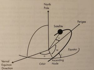
Source: Courtesy of (Adamy D. L., Space Electronic Warfare, 2021)
From the orbital elements, it is possible to compute the position and velocity of the satellite.
Kepler’s Third Law states that the relationship between the size of the orbit and its period is defined by:
a3 = CP2; therefore, C = a3/ P2. Eq. 10-1
Where:
a = the semi-major axis of the orbit ellipse,
C = a constant, and
P = the orbit period.
Example: If a Satellite circles the Earth every 1.5 hours and has an altitude of 281.4-km-high (or a radius from the center of the Earth of 6,653 km, then C is calculated as; 6,653 km3/90 min2 = 36,355.285 km per min2
Table 10-2 Shows the altitude of a circular Earth satellite versus the period of its orbit for satellites with periods of 1.5 hours to 9 hours.
Altitude and Semi-Major Axis of Circular Orbits Versus the Satellite Period
| p(min) | h(km) | α(km) | p(min) | h(km) | α(km) |
| 90 | 281 | 6652 | 330 | 9447 | 15818 |
| 105 | 1001 | 7372 | 345 | 9923 | 16294 |
| 120 | 1688 | 8059 | 360 | 10392 | 16763 |
| 135 | 2346 | 8717 | 375 | 10854 | 17225 |
| 150 | 2980 | 9351 | 390 | 11311 | 17682 |
| 165 | 3594 | 9965 | 405 | 11761 | 18132 |
| 180 | 4189 | 10560 | 420 | 12206 | 18577 |
| 195 | 4768 | 11139 | 435 | 12646 | 19017 |
| 210 | 5332 | 11703 | 450 | 13081 | 19452 |
| 225 | 5883 | 12254 | 465 | 13510 | 19881 |
| 240 | 6422 | 12793 | 480 | 13936 | 20307 |
| 255 | 6949 | 13320 | 495 | 14357 | 20728 |
| 270 | 7466 | 13837 | 510 | 14773 | 21144 |
| 285 | 7974 | 14345 | 525 | 15186 | 21557 |
| 300 | 8473 | 14844 | 540 | 15595 | 21966 |
| 315 | 8964 | 15350 | – | – | – |
Source: (Adamy D. L., Space Electronic Warfare, 2021)
Figure 10-2 Altitude of a Circular Satellite is a Function of its Orbital Period
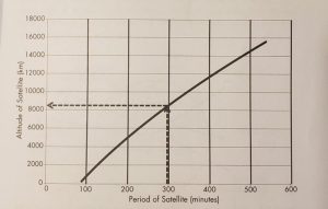
Source courtesy of (Adamy D. L., Space Electronic Warfare, 2021)
LOOK ANGLES
An Earth Trace is the locus of latitude and longitude of the SVP as the satellite moves through its orbit. Note: The SVP is the point on the Earth’s surface directly below the satellite. This point intersects the line from the center of the Earth to the satellite with the surface of the Earth. LEO (low earth orbits) determines the moment-to-moment area of the Earth that the satellite sees. It also allows us to calculate the look angles and range of the satellite from a specified point on (or above) the Earth at any specified time. See Figure 10-3.
Using the six elements of Ephemeris, the exact location of a satellite can be calculated at any time. For example, the Earth Trace of a satellite with a 90-minute orbital period will move West by 22.56 longitude degrees for each subsequent orbit. Example: (90-minute orbital Period / 1463 sidereal day, minutes) x 360 deg = 22.56 deg. Earth Traces are very important in using emerging space technologies for humanitarian purposes. They give policymakers new approaches to feeding populations, increasing crop efficiencies, routing navigation, improving cattle feeding, and building more effective fire barriers. (Nichols & al, Space Systems: Emerging Technologies and Operations, 2022)
Figure 10-3 Earth Trace of the satellite is the path of the SVP over the Earth’s surface in a Polar view.
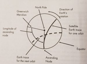
Source: Courtesy of (Adamy D. L., Space Electronic Warfare, 2021)
Where: (SVP = Sub-vehicle point) and is the intersection of a line from the center of the Earth to the satellite with the Earth’s surface
The Earth area over which a satellite can send or receive signals to and from the Earth-based stations during each orbit depends on the satellite’s altitude and the beam width and orientation of antennas on the satellite. If a satellite is placed in polar orbit, its orbit has 90֩ inclination and will, therefore, eventually provide complete coverage of the surface of the Earth.
Figure 10-4 Earth Trace of a satellite is the path of the SVP over the Earth’s surface in an equatorial view.
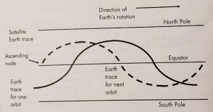
Source: Courtesy of (Adamy D. L., Space Electronic Warfare, 2021)
A synchronous satellite has an SVP that stays in one location on the Earth’s surface. This requires that its orbital period be one sidereal day (i.e., 1,436 minutes). Another requirement for a fixed SVP is that the orbit has an 0° inclination. That would place it directly on the border.
Figure 10-5 shows a sample calculation of the range of a synchronous satellite based on a semi-major axis of 42,166 km. “In a circular orbit, the satellite’s height will be 35,795 km. The maximum range can be calculated from the Earth’s surface station (ESS) to the synchronous satellite with a circular orbit. The diagram is a planer triangle in the plane containing the Earth’s ESS, satellite, and center. The ESS sees the satellite at 0 deg elevation. The minimum and maximum range values for the satellite to the ground link are 35,795 km and 41,682 km. The shorter range applies if the satellite is directly overhead, and the maximum range is for the satellite to the horizon as shown.” (Adamy D. L., Space Electronic Warfare, 2021)
Figure 10-5 Example calculation: Maximum range to a synchronous satellite on the horizon is 41,759 km by Kepler’s Laws. Link loss for a 2 GHz signal would be from 189.5 to 190.9 dB
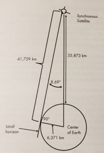
Source: Courtesy of (Adamy D. L., Space Electronic Warfare, 2021)
LOCATION OF THREAT TO SATELLITE
The location of a threat from the satellite is defined in terms of the azimuth and elevation of a vector from the satellite that points at the threat location and the range between the satellite and the threat. The vector points information for a satellite antenna aimed at the threat. An EW system on the satellite will either intercept signals from a threat transmitter or transmit jamming or spoofing signals to a threat receiver at the considered location. (Adamy D. L., Space Electronic Warfare, 2021) (Nichols R. &., 2022) See Figure 10-6.
Figure 10-6 The azimuth and elevation angle from the nadir defines the direction of a threat to a satellite.
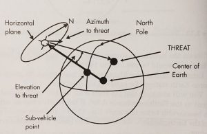
Source: Courtesy of (Adamy D. L., Space Electronic Warfare, 2021)
Where: the azimuth is the angle between true North and the threat location in a plane at the satellite perpendicular to the vector from the SVP. The elevation is the angle between the SVP and the threat. The nadir is defined as the point on the celestial sphere directly below an observer.
CALCULATING LOOK ANGLES
For the azimuth calculation, we need to consider the spherical triangle. Consider Figures 10-7 and 10-8.
Figure 10-7 A spherical triangle is formed between the North Pole, the SVP, and the Threat location.
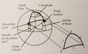
Source: Courtesy of (Adamy D. L., Space Electronic Warfare, 2021)
The elevation from the nadir and range to a threat from a satellite can be determined from the plane triangle defined by the satellite, the threat, and the center of the Earth. For example, Set E is at the satellite, F is at the threat, and G is at the center of the Earth. Side e is the radius of the Earth (6,371 km). Side f is the semi-major axis (the radius of the Earth plus the satellite altitude = 10,560 km), angle G is side a from the spherical triangle above (21.57°), and side g is the propagation distance between the satellite and the threat. We use the law of cosines for plane triangles to calculate the relationships – specifically the propagation distance between the satellite and the threat; to wit:
g2 = e2 + f2 – 2ef cos(G) Eq. 10-2
Figure 10-8 The elevation from the nadir and range to a threat from a satellite can be determined from the plane triangle defined by the satellite, threat, and the center of the Earth.
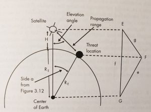
Source: Courtesy of (Adamy D. L., Space Electronic Warfare, 2021)
PROPAGATION LOSS MODELS
Messages travel (propagate) through Space as radio waves (electromagnetic waves). This is similar to the radio waves we receive with our car radio. Each spacecraft has a transmitter and receiver for radio waves and a way of interpreting the information received and acting on it. Electromagnetic waves are unlike sound waves because they do not need molecules to travel. This means electromagnetic waves can travel through air, solid objects, and Space. This is how astronauts on spacewalks use radios to communicate.
Space wave propagation refers to the satellite signals of radio transmitted freely through the Earth’s atmosphere. Space wave propagation refers to the radio waves transmitted from the antenna to propagate (travel) along Space to reach the receiver antenna.
It is not a clean transmission because of the long distances to satellites. There are losses in the link between the antenna and the receiver. (R.K. Nichols & Lekkas, 2002)
(Adamy D. L., Space Electronic Warfare, 2021) presents several propagation loss models within the atmosphere based on a clear or obstructed path and Fresnel zone distance. Refer to Table 10-3. These models are LOS (free space loss or spreading loss), two-ray propagation for phase cancellation, and KED (knife-edge loss). Adamy also considers atmospheric, rain, and fog losses.
Table 10-3 Selection of Appropriate Propagation Loss Model
| Clear propagation path | Low-frequency, wide beams near the ground | Link longer than Fresnel-zone distance | Use two-ray model |
| Link shorter than Fresnel-zone distance | Use LOS model | ||
| Hight-frequency, narrow-beams | Far from ground | Use LOS model | |
| Propagation path obstructed by terrain. | Calculate additional loss from the KED model. | ||
Source: Reprinted from Table 4.1 courtesy of (Adamy D. L., Space Electronic Warfare, 2021)
RECEIVED POWER AT THE RECEIVER
When radio transmission and propagation is to or from an Earth satellite, there are special considerations due to the nature of Space, losses due to extreme long range, and the geometry of the links. The 10-3 formula gives the received power to the receiver:
PR = ERP – L + GR Eq. 10-3
Where:
PR– received signal power in dBm
ERP– the effective radiated power, in dBm
L – losses from all causes between transmitting and receiving antennas in dBm
GR – receiver antenna gain in dBm
The total path loss to or from a satellite includes LOS loss, atmospheric loss, antenna misalignment loss, polarization loss, and rain loss. (Adamy D. L., Space Electronic Warfare, 2021) [3]
ONE-WAY LINK EQUATION
The one-way link equation gives the received power PR in terms of the other link components (in decibel units). It is:
PR = PT + GT – L + GR Eq. 10-4
Where:
PR – received signal power in dBm
PT – transmitter output power in dBm
GT – transmitter antenna gain in dBm
L – link losses from all causes as a positive number in dBm
GR – receiver antenna gain in dBm
In linear (non-decibel units), this formula is:
PR = ( PT GT GR ) / L Eq. 10-5
It is assumed that all link losses from propagation are between isotropic antennas (unity gain, 0-dB gain). (Adamy D. L., Space Electronic Warfare, 2021)
INTERCEPTED COMMUNICATION SIGNAL
When a communication signal is intercepted, there are two links to consider: the transmitter to intercept the receiver link and the transmitter to desired receiver link. Refer to Figure 10-9.
Figure 10-9 Intercepted Communication Signal
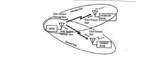
Source: Reprinted /modified from Figure 4-3 courtesy of (Adamy D. L., Space Electronic Warfare, 2021)
JAMMED / SPOOFED COMMUNICATIONS SIGNAL
When a communication signal is jammed or spoofed, there is a link from the desired transmitter to the receiver and a link from a jammer or spoofer to the receiver. (Adamy D. L., Space Electronic Warfare, 2021) [4] Refer to Figure 10-10.
Figure 10-10 Jammed / Spoofed Communications Signal
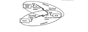
Source: Reprinted/modified from Figure 4-4 courtesy of (Adamy D. L., Space Electronic Warfare, 2021)
SATELLITE LINKS
Satellites are, by nature, remote from the ground and must be connected by links. Uplink and downlink geometry is a complex set of calculations related to satellite position, North Pole, longitudes, latitudes, sub-vehicle points (SVP), Center of Earth, ground station, Equator, Greenwich Meridian, Azimuth to the ground station, satellite movement in the horizontal plane, satellite payloads, radar bore sights, and hostile target detection, all wrapped up in complex orbital and spherical geometry calculations. (Adamy D. L., Space Electronic Warfare, 2021) spends four challenging chapters on this subject.
Uplinks have transmitters on or near Earth’s surface and receivers in the satellite. The uplink equation is 10-4. L is the in that equation is Link Losses. Table 10-4 shows the various Uplink Losses.
Table 10-4 Uplink Losses
| Loss | Description |
| Transmit antenna misalignment | Reduction from boresight gain at the offset angle from the direction to the satellite |
| Receiving antenna misalignment | Reduction from boresight gain at the offset angle from the direction to the ground-based transmitter |
| Space loss | LOS loss assuming that both the transmit and receive antennas are isotropic |
| Atmospheric loss | Atmospheric attenuation at the elevation angle through the atmosphere from the ground transmitter |
| Rain loss | Rain attenuation over the part of the link that passes through the rain |
Source: Courtesy of (Adamy D. L., Space Electronic Warfare, 2021)
Command links control functions of the satellite, such as its orientation, payloads, and synchronization of multiple payloads. (Adamy D. L., Space Electronic Warfare, 2021)
Intercept links (satellite-borne system) are defined from the hostile transmitter to the satellite payload receiver
The power received by the satellite payload receiver in the presence of a hostile transmitter is given by equation 10-6:
PR = PT + GT – Link Losses + GR Eq. 10-6
Where:
PR – Power received by satellite payload receiver
PT – Hostile transmitter output power
GT – Boresight gain of the hostile transmitter
Link Losses – Table 10-4
GR – Boresight gain of satellite payload receiving antenna
Downlinks from the satellite to the ground can be the satellite’s control station, to other receivers at stations that require information that the satellite has gathered, or to hostile receivers that intercept the satellite downlink. They can also be to hostile receivers that are jammed or spoofed from the satellite. (Adamy D. L., EW 103: Tactical Battlefield Communications Electronic Warfare, 2009) (Nichols R. &., 2022)
The downlink equation is given by 10-7.
PR = PT + GT – Link Losses + GR Eq. 10-7
Where:
PR – Power received by the ground-based receiver or hostile receiver
PT – Output power of the satellite’s transmitter
GT – Boresight gain of satellite’s antenna
Link Losses – Table 10-4
GR – Boresight gain of ground-based receiving antenna
Table 10-5 Downlink Losses
| Loss | Description |
| Transmit antenna misalignment | Reduction from boresight gain at the offset angle from the direction to the ground-based receiver |
| Receiving antenna misalignment | Reduction from boresight gain at the offset angle from the direction to the satellite |
| Space loss | LOS loss assuming that both the transmit and receive antennas are isotropic |
| Atmospheric loss | Atmospheric attenuation at the elevation angle through the atmosphere from the ground-based receiver |
| Rain loss | Rain attenuation over the part of the link that passes through the rain |
Source: Courtesy of (Adamy D. L., Space Electronic Warfare, 2021)
User data links – a satellite may collect usage data for many users. User data links receive satellite data directly. Users may not be authorized to receive all the data available /collected from /by the satellite. The ground station may edit the data and retransmitted back to the satellite and back again to users. (Adamy D. L., Space Electronic Warfare, 2021)
Jamming Links – ground communication links and satellite radar links can be jammed. The target receiver can either be on the Earth’s surface or in an aircraft or UAS flying above the Earth. Like intercept links, the received power into the target receiver is calculated by the same formula. Still, the transmitted power is from the satellite jammer, and the received power is at the target receiver.
The Jammed link equation is given by 10-8.
PR = PT + GT – Link Losses + GR Eq. 10-8
Where:
PR – Power received by the target receiver
PT – Satellite jammer output power
GT – Boresight gain of jammer transmitter
Link Losses – Table 10-5
GR – Boresight gain of target receiver antenna
LINK VULNERABILITY TO EW: SPACE-RELATED LOSSES, INTERCEPT JAMMING & SPOOFING
Satellites are from Earth but present excellent loss of signal (LOS) from a large part of the Earth’s surface. As reported previously, satellite links are highly susceptible to three kinds of hostile activity. Signals from satellites can be intercepted, and strong hostile transmissions can be jamming signals, interfering with uplink or downlink signals to prevent proper reception. (Adamy D. L., Space Electronic Warfare, 2021) They can also be spoofing signals that cause the satellite to interpret them as functional commands that are harmful or transmit useless positional data. This section and the following will focus heavily on spoofing and the downlink interpretation of false signals in GNSS/GPS/ADS-B receivers. (Nichols R. &., 2022)
Figure 10-11 shows a successful intercept of a satellite signal. Successful intercept gives the hostile receiver a high-quality signal to recover important information. A ground-based jammer operating against a satellite uplink transmits to the link receiver in the satellite. The ground station and the jammer must be above the horizon from the satellite. The received signals are intended for the receiver in the satellite control station (GCS) or another authorized receiver. There is a separate link to any hostile receiver. (Adamy D. L., EW 103: Tactical Battlefield Communications Electronic Warfare, 2009) (Adamy D. L., Space Electronic Warfare, 2021)
Successful spoofing places a strong enough signal into a satellite link receiver to cause the satellite or its payload to accept it as a valid command. Command spoofing could cause the satellite to perform a maneuver that ends the mission or put the payload in an unusable state. (Adamy D. L., Space Electronic Warfare, 2021) (Nichols R. &., 2022)
Figure 10-12 shows a successful spoofing of a satellite signal. A ground-based spoofer operating against a satellite uplink transmits to the link receiver in the satellite. The ground station and the jammer must be above the horizon from the satellite.[5]
Figure 10-11 Successful Intercept
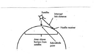
Source: Figure 10-32 Modified from Figure 7.1 Courtesy of (Adamy D. L., Space Electronic Warfare, 2021)
Figure 10-12 Successful Spoofing
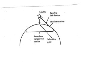
Source: Figure 10-12 Modified from Figure 7.2 Courtesy of (Adamy D. L., Space Electronic Warfare, 2021)
SPACE-RELATED LINK LOSSES
Any attack on a satellite link may involve single or multiple links. Each link is subject to transmission losses, including LOS, atmospheric, antenna misalignment, rain, and polarization losses.
An intercept link is separate from the intended command and data links. It goes from the satellite’s link transmitter (onboard or at GCS) to a hostile receiver. The quality of the intercept is judged by the Signal to Noise (S/N) ratio achieved in the hostile receiver. (Adamy D. L., Space Electronic Warfare, 2021)
A spoofing link goes from the hostile transmitter to a satellite link receiver. This receiver is generally on the satellite. The spoofing signal’s purpose is to cause it to function improperly, but if the spoofer is in the GCS, the purpose is to invalidate the data – especially localization data. (Nichols R. &., 2022) (Adamy D. L., EW 104: EW against a new generation of threats, 2015)
Jamming of any satellite link is communications jamming. Jamming effectiveness is defined in terms of the Jamming-to-Signal ratio (J/S) that it causes. It is calculated from the following formula:
J / S = ERPJ – ERPS – LOSSJ + LOSSS + GRJ – GR Eq. 10-9
Where:
J / S = Jamming-to-signal ratio in decibels
ERPJ = Effective radiated power (ERP) of jamming transmitter toward the target receiver in dBm
ERPS = ERP of the desired signal toward the receiver in dBm
LOSSJ = Transmission loss from the jammer to target a receiver in dBm
LOSSS = Transmission loss from transmitter to target a receiver in decibels
GRJ = Gain of receiving antenna in the direction of a jammer in decibels
GR = Gain of receiving antenna toward transmitter in decibels
The last two terms cancel each other if the target receiver has a non-directional antenna.
(Adamy D. L., Space Electronic Warfare, 2021) in his textbook, he presents and solves detailed examples of intercepting, jamming, and spoofing uplinks and downlinks. [6] [7]
GPS/GNSS SPOOFING -PRACTICAL SPOOFING
GPS spoofing detection and mitigation for GNSS / GPS using the ECD algorithm will be addressed. GPS spoofing of ADS-B systems was covered in detail (Nichols R. &., 2022).[8] Recognize that ADS-B is a subset of the larger receiver localization problem. Solutions that apply to the larger vector space, GNSS / GPS, also are valid for the subset, ADS-B, if computational hardware is available. GPS spoofing is a reasonably well-researched topic. Many methods have been proposed to detect and mitigate spoofing. The lion’s share of the research focuses on detecting spoofing attacks. Methods of spoofing mitigation are often specialized or computationally burdensome. Civilian COTS anti-spoofing countermeasures are rare. Nevertheless, much better technology is available to Detect, Mitigate and Recover Spoofed satellite signals – even those with a precursor Jamming attack. It is called ECD.
ECD: EICHELBERGER COLLECTIVE DETECTION
This section covers the brilliant value-added research by Dr. Manuel Eichelberger on the detection, mitigation, and recovery of GPS-spoofed signals. (Eichelberger, 2019) ECD implementation and evaluation show that with some modifications, the robustness of collective detection (CD) can be exploited to mitigate spoofing attacks. (Eichelberger, 2019) shows that multiple locations, including the actual one, can be recovered from scenarios where several signals are present. [9] [10]
ECD does not track signals. It works with signal snapshots. It is suitable for snapshot receivers, a new low-power GPS receiver class. (M. Eichelberger, 2019) (J. Liu & et.al., 2012)
SPOOFING
Threats and weaknesses show that large damages (even fatal or catastrophic) can be caused by transmitting forged GPS signals. False signal generators may cost only a few hundred dollars of software and hardware. (Humphreys & al., 2008)
A GPS receiver computing its location wrongly or even failing to estimate any location at all can have different causes. Wrong localization solutions come from 1) a low signal-to-noise ratio (SNR) of the signal (examples: inside a building or below trees in a canyon), 2) reflected signals in multipath scenarios, or 3) deliberately spoofed signals. (Eichelberger, 2019) discusses mitigating low SNR and multipath reflected signals. Signal spoofing (#3) is the most difficult case since the attacker can freely choose the signal power and delays for each satellite individually. (Eichelberger, 2019)
Before discussing ECD – Collective detection maximum likelihood localization approach (Eichelberger, 2019), it is best to step back and briefly discuss GPS signals, classical GPS receivers, A-GPS, and snapshot receivers. Then the ECD approach to spoofing will show some real power by comparison. Power is defined as both enhanced spoofing detection and mitigation capabilities. [11]
GPS SIGNAL
The GPS consists of control, space, and user segments. The space segment contains 24 orbiting satellites. The network monitor stations, GCS, and antennas comprise the control segment. The third and most important are the receivers, which comprise the user segment. (USGPO, 2021)
Satellites transmit signals in different frequency bands. These include the L1 and L2 frequency bands at 1.57542 GHz and 1.2276 GHz. (DoD, 2008) Signals from different satellites may be distinguished and extracted from background noise using code division multiple access protocols (CDMA). (DoD, 2008) Each satellite has a unique course/acquisition code (C/A) of 1023 bits. The C/A codes are PRN sequences transmitted at 10.23 MHz, which repeats every millisecond. The C /A code is merged using an XOR before being with the L1 or L2 carrier. The data broadcast has a timestamp called HOW, which is used to compute the location of the satellite when the packet was transmitted. The receiver needs accurate orbital information ( aka Ephemeris) about the satellite, which changes over time. The timestamp is broadcast every six seconds; the ephemeris data can only be received if the receiver can decode at least 30 seconds of the signal.[12] (Eichelberger, 2019)
CLASSIC RECEIVERS
Classical GPS receivers use three stages when obtaining a location fix. They are Acquisition, Tracking, and localization.
Acquisition. The relative speed between the satellite and receiver introduces a significant Doppler shift to the carrier frequency. [13] GPS receiver locates the set of available satellites. This is achieved by correlating the received signal with the satellites’. Since satellites move at considerable speeds. The signal frequency is affected by a Doppler shift. So, the receiver must correlate the received signal with C/ A codes with different Doppler shifts. (Eichelberger, 2019)
Tracking. After a set of satellites has been acquired, the data contained in the broadcast signal is decoded. Doppler shifts and C /A code phase are tracked using tracking loops. After the receiver obtains the ephemeris data and HOW timestamps from at least four satellites, it can start to compute its location. (Eichelberger, 2019)
Localization. Localization in GPS is achieved using signal time of flight (ToF) measurements. ToFs are the difference between the arrival times of the HOW timestamps decoded in the tracking stage of the receiver and those signal transmission timestamps themselves. [14] The local time at the receiver is unknown, and the localization is done using pseudo ranges. The receiver location is usually found using least-squares optimization. (Eichelberger, 2019) (Wikipedia, 2021)
A main disadvantage of GPS is the low bit rate of the navigation data encoded in the signals transmitted by the satellites. The minimal data necessary to compute a location fix, which includes the ephemerides of the satellites, repeats only every 30 seconds. [15]
SNAPSHOT RECEIVERS
Snapshot receivers aim at the remaining latency that results from the transmission of timestamps from satellites every six seconds. Snapshot receivers can determine the ranges to the satellite modulo 1 ms, which corresponds to 300 km.
COLLECTIVE DETECTION
Collective Detection (CD) is a maximum likelihood snapshot receiver localization method, which does not determine the arrival time for each satellite but combines all the available information and decides only at the end of the computation. [16] This technique is critical to the (Eichelberger, 2019) invention to mitigate spoofing attacks on GPS /GNSS or ADS-B. CD can tolerate a few low-quality satellite signals and is more robust than CTN. CD requires much computational power. CD can be sped up by a branch and bound approach, which reduces the computational power per location fix to the order of one second, even for uncertainties of 100 km and a minute. CD improvements and research has been plentiful. (Eichelberger, 2019) (J.Liu & et.al., 2012) (Axelrod & al, 2011) (P. Bissag, 2017)
ECD
Dr. Manuel Eichelberger’s CD – Collective detection maximum likelihood localization approach method not only can detect spoofing attacks but also mitigate them! The ECD approach is a robust algorithm to mitigate spoofing. ECD can differentiate closer differences between the correct and spoofed locations than previously known approaches. (Eichelberger, 2019) COTS has little spoofing integrated defenses. Military receivers use symmetrically encrypted GPS signals, subject to a “replay” attack with a small delay to confuse receivers.
ECD solves even the toughest type of GPS spoofing attack consisting of spoofed signals with power levels similar to the authentic ones.[17] (Wesson, 2014) For each location fix, the ECD approach uses only a few milliseconds of raw GPS signals, so-called snapshots. This enables offloading of the computation into the Cloud, which allows knowledge of observed attacks. [18] Existing spoofing mitigation methods require a constant stream of GPS signals and tracking those signals over time. Computational load increases because fake signals must be detected, removed, or bypassed. (Eichelberger, 2019)
SPOOFING TECHNIQUES
According to (Haider & Khalid, 2016), there are three common GPS Spoofing techniques with different sophistication levels. They are simplistic, intermediate, and sophisticated. (Humphreys & al., 2008)
The simplistic spoofing attack is the most commonly used technique to spoof GPS receivers. It only requires a COTS GPS signal simulator, amplifier, and antenna to broadcast signals to the GPS receiver. It was performed successfully by Los Almos National Laboratory in 2002. (Warner & Johnson, 2002) Simplistic spoofing attacks can be expensive as the GPS simulator can run $400K and is heavy (not mobile). The available GPS signal and detection do not synchronize simulator signals is easy.
In the intermediate spoofing attack, the spoofing component consists of a GPS receiver to receive a genuine GPS signal and a spoofing device to transmit a fake GPS signal. The idea is to estimate the target receiver antenna position and velocity and then broadcast a fake signal relative to the genuine GPS signal. This spoofing attack is difficult to detect and can be partially prevented using an IMU. (Humphreys & al., 2008)
In sophisticated spoofing attacks, multiple receiver-spoofer devices target the GPS receiver from different angles and directions. In this scenario, the angle-of-attack defense against GPS spoofing in which the reception angle is monitored to detect spoofing fails. The only known defense successful against such an attack is cryptographic authentication. (Humphreys & al., 2008) [19]
Note that prior research on spoofing was to exclude fake signals and focus on a single satellite. ECD includes the fake signal on a minimum of four satellites and then progressively / selectively eliminates their effect until the real weaker GPS signals become apparent. (Eichelberger, 2019)
GPS SIGNAL JAMMING AS A PRECURSOR TO SPOOFING ATTACK
The easiest way to prevent a receiver from finding a GPS location is by jamming the GPS frequency band. GPS signals are weak and require sophisticated processing to be found. Satellite signal jamming considerably worsens the signal-to-noise ratio (SNR) of the satellite signal acquisition results. ECD algorithms achieve a better SNR than classical receivers and tolerate more noise or stronger jamming. (Eichelberger, 2019)
A jammed receiver is less likely to detect spoofing since the original signals cannot be accurately determined. The receiver tries to acquire any satellite signals it can find. The attacker only needs to send a set of valid GPS satellite signals stronger than the noise floor without synchronizing with the authentic signals. [20] (Eichelberger, 2019)
There is a more powerful and subtle attack on the jammed signal. To spoof the receiver successfully, the spoofer can send satellite signals with adjusted power levels synchronized to the authentic signals. (Eichelberger, 2019) So even if the receiver has countermeasures to differentiate the jamming, the spoofer signals will be accepted as authentic. (Nichols R. K., 2020)
TWO ROBUST GPS SIGNAL SPOOFING ATTACKS AND ECD
Two of the most powerful GPS signal spoofing attacks are Seamless Satellite-Lock Takeover (SSLT) and Navigation Data Modification (NDM). How does ECD perform against these?
SEAMLESS SATELLITE-LOCK TAKEOVER (SSLT)
The most powerful attack is a seamless satellite-lock takeover. In such an attack, the original and counterfeit signals are nearly identical concerning the satellite code, navigation data, code phase, transmission frequency, and received power. This requires the attacker to know the location of the spoofed device precisely so that ToF and power losses over a distance can be factored in. After matching the spoofed signals with the authentic ones, the spoofer can send its signals with a small power advantage to trick the receiver into tracking those instead of the authentic signals. A classical receiver without spoofing countermeasures, like tracking multiple peaks, cannot mitigate or detect the SSLT attack, and there is no indication of interruption of the receiver’s signal tracking. (Eichelberger, 2019)
NAVIGATION DATA MODIFICATION (NDM)
An attacker has two attack vectors: modifying the signal’s code phase or altering the navigation data—the former changes the signal arrival time measurements. The latter affects the perceived satellite locations. Both influence the calculated receiver location. ECD works with snapshot GPS receivers and is not vulnerable to NDM changes as they fetch information from other sources like the Internet. ECD deals with modified, wireless GPS signals.
ECD ALGORITHM DESIGN
ECD is aimed at single-antenna receivers. Its spoofing mitigation algorithm object is to identify all likely localization solutions. It is based on CD because 1) CD has improved noise tolerance compared to classical receivers, 2) CD is suitable for snapshot receivers, 3) CD is not susceptible to navigation data modifications, and 4) CD computes a location likelihood distribution which can reveal all likely receiver locations including the actual location, independent of the number of spoofed and multipath signals. ECD avoids all the spoofing pitfalls and signal selection problems by joining and transforming all signals into a location likelihood distribution. Therefore, it defeats the top two GPS spoofing signal attacks. (Eichelberger, 2019)
Regarding the fourth point, spoofing and multipath signals are similar from a receiver’s perspective. Both result in several observed signals from the same satellite. The difference is that multipath signals have a delay dependent on the environment while spoofing signals can be crafted to yield a consistent localization solution at the receiver. To detect spoofing and multipath signals, classical receivers can be modified to track an arbitrary number of signals per satellite instead of only one. (S.A.Shaukat & al., 2016) In such a receiver, the set of authentic signals – one signal from each satellite – would have to be correctly identified. Any selection of signals can be checked for consistency by verifying that the resulting residual error of the localization algorithm is very small. This is a combinatorically difficult problem. For n satellites and m transmitted sets of spoofed signals, there are (m+ 1) n possibilities for the receiver to select a set of signals. Only m + 1 of those will result in a consistent localization solution representing the actual location and m spoofed locations. ECD avoids this signal selection problem by joining and transforming all signals into a location likelihood distribution. (Eichelberger, 2019)
ECD only shows consistent signals since just a few overlapping (synced) signals for some location hypotheses do not accumulate a significant likelihood. All plausible receiver locations – given the observed signals – have a high likelihood. Finding these locations in four dimensions, Space and time, is computationally expensive. (Bissig & Wattenhoffer, 2017) (Eichelberger, 2019) describes improved Branch and Bound implementations to reduce the calculation load and find plausible receiver locations.[21]
SIGNALS INTELLIGENCE (SIGINT), EW, and EP
Satellites are perfect for implementing SIGINT and EW, depending on the specific situation and activity. [22]
This final section will cover the key formulas for successful intercept, the intercept link equation, communications jamming (by extension spoofing), and communications EP (electronic protection). Radar Jamming will not be covered but can be found in (Adamy D. L., EW 103: Tactical Battlefield Communications Electronic Warfare, 2009) and (Adamy D. L., EW 104: EW against a new generation of threats, 2015)
SUCCESSFUL INTERCEPT
Figure 10-13 shows an intercept link.
Figure 10-13 Intercept Link
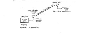
Source: Courtesy of and modified from Figure A-1, p200 in (Adamy D. L., Space Electronic Warfare, 2021)
The parameters of this link are the hostile transmitter power, the transmit antenna gain in the direction of the intercept receiver, the distance to the intercept receiver ( the satellite), and the antenna configuration at the intercept site. (Adamy D. L., Space Electronic Warfare, 2021)
A successful intercept occurs when a receiver in the satellite receives a hostile signal with enough quality to recover the information carried by the signal. For communication signals, transmission frequency, modulation, the type of encryption employed, the signal’s timing, or the signal’s location can constitute hostile level quality.[23] Modulation, voice imagery, and data can also constitute hostile quality. [24] (Adamy D. L., Space Electronic Warfare, 2021)
THE INTERCEPT LINK EQUATION
In order to intercept a signal, the received signal strength must exceed the sensitivity level of the receiver. The Sensitivity (S) is the weakest signal the receiver can receive and still extract the required information from that signal. We need to budget for the power out of the receiving antenna. The intercept link equation is (Adamy D. L., Space Electronic Warfare, 2021):
PR = ERP – Loss + GR Eq. 10-10
Where:
PR – Power out of the receiving antenna, dBm,
ERP – Effective radiated power of the Hostile signal to be intercepted,
Loss – Loss is the sum of all the losses between the Hostile transmitter’s antenna and the intercept receiver’s antenna ( in decibels), (L)
GR – is the receiving antenna gain.
S/L – Signal to Noise Level measure in some minimum, -dB
Received signal quality is normally stated in a signal-to-noise ratio or minimum level of combined noise factors to overcome. This is the received signal level at the output of the receiving antenna divided by the noise level at the same point in the receiver system. The minimum discernable signal (MDS) is the received signal level when the signal power equals the noise power. (Adamy D. L., Space Electronic Warfare, 2021)
Communications Jamming and radar jamming plus EP (electronic protection measures) are covered in (Adamy D. L., EW 103: Tactical Battlefield Communications Electronic Warfare, 2009) (Adamy D. L., EW 104: EW against a new generation of threats, 2015) (Nichols R. &., 2022). They are beyond the scope of this chapter.
CONCLUSIONS
For purposes of this chapter and Chapter 10, we have arbitrarily chosen three general altitude reference points: 1) Earth’s surface (ground zero); 2) The maximum distance to Geosynchronous and Geostationary Satellites from the Earth’s surface(22,236 mi); and 3) Deep Space beyond the maximum altitude for Satellites (>22,236 mi). (High Earth Orbit, 2023). Satellites are from Earth and present an excellent LOS from many of Earth’s surfaces. Satellites are vulnerable and susceptible to three types of hostile activity: Signal Interception, Signal Jamming, or interference with uplink or downlink signals and spoofing signals to make the signals function incorrectly. Our main concentration has been on EW, with a secondary interest in spoofing signals. We have barely skimmed the topics of Orbital Mechanics (the language of Satellites), signal interception, jamming, spoofing, and ECD. However, it should give us enough of a flavor of the EW purview to extend our thinking into Deep Space Warfare (Chapter 12).
REFERENCES
Adamy, D. (2001). EW 101: A First Course in Electronic Warfare. Boston: Artech House.
Adamy, D. L. (2004). EW 102 A Second Course in Electronic Warfare. Norwood, MA: Artech House.
Adamy, D. L. (2009). EW 103: Tactical Battlefield Communications Electronic Warfare. Norwood, MA: Artech House.
Adamy, D. L. (2011 (2281st edition) ). Electronic Warfare Pocket Guide. Raleigh, NC: SCItech.
Adamy, D. L. (2015). EW 104: EW against a new generation of threats. Norwood, MA: Artech House.
Adamy, D. L. (2021). Space Electronic Warfare. Norwood, MA: Artech House.
Axelrod, P., & al, e. (2011). Collective Detection and Direct Positioning Using Multiple GNSS Satellites. Navigation, pp. 58(4): 305-321.
Bissig, P., & Wattenhoffer, M. E. (2017). Fast & Robust GPS Fix using 1 millisecond of data . 16 ACM / IEEE Int Conf on Information Processing in Sensor Networks (pp. 223-234). Pittsburg, PA: IPSN.
Christian Wolff. (2022). Radar and Electronic Warfare Pocket Guide. Munich, Germany: Rhodes & Schwartz.
Diggelen, F. V. (2009). A-GPS: Assisted GPS, GNSS, and SBAS. NYC: Artech House.
DoD. (2008). Global Positioning System Performance Standard 4th edition (GPS SPS PS). Washington, DC: DoD.
Eichelberger, M. (2019). Robust Global Localization using GPS and Aircraft Signals. Zurich, Switzerland: Free Space Publishing, DISS. ETH No 26089.
GPSPATRON. (2022, July 9). GNSS Interference in wildlife. Retrieved from GPSPATRON.com: https://GPSPATRON.com/gnss-interference-from-wildlife/
Haider, Z., & Khalid, &. S. (2016). Survey of Effective GPS Spoofing Countermeasures. 6th Intern. Ann Conf on Innovative Computing Technology (INTECH 2016) (pp. 573-577). IEEE 978-1-5090-3/16.
High Earth Orbit. (2023, Feb 1). Retrieved from Wikipedia: en.m.wikipedia.org
Humphreys, T., & al., e. (2008). Assessing the spoofing threat: Development of a portable GPS civilian spoofer. In Radionavigation Laboratory Conf. Proc.
IS-GPS-200G. (2013, September 24). IS-GPS-200H, GLOBAL POSITIONING SYSTEMS DIRECTORATE SYSTEMS ENGINEERING & INTEGRATION: INTERFACE SPECIFICATION IS-GPS-200 – NAVSTAR GPS SPACE SEGMENT/NAVIGATION USER INTERFACES (24-SEP-2013). Retrieved from http://everyspec.com/: http://everyspec.com/MISC/IS-GPS-200H_53530/
J. Liu, & et.al. (2012, November). Energy Efficient GPS Sensing with Cloud Offloading. Proceedings of 10 ACM Conference on Embedded Networked Sensor Signals (SenSys) , pp. 85-89.
M. Eichelberger, v. H. (2019). Multi-year GPS tracking using a coin cell. In Proc.of 20th Inter.Workshop on Mobile Computing Systems & Applications ACM , 141-146.
Nichols, R. &. (2022). Space Electronic Warfare, Jamming Spoofing and ECD. In R. Nichols, & e. al, Space Systems: Emerging Technologies and Operations (pp. 112 – 232). Manhattan, KS: New Prairie Press #47.
Nichols, R. K. (2020). Counter Unmanned Aircraft Systems Technologies & Operations. Manhattan, KS: www.newprairiepress.org/ebooks/31.
Nichols, R. K., & Sincavage, S. M. (2022). DRONE DELIVERY OF CBNRECy – DEW WEAPONS Emerging Threats of Mini-Weapons of Mass Destruction and Disruption (WMDD). Manhattan, KS: New Prairie Press #46.
Nichols, R. K.-P. (2019). Unmanned Aircraft Systems in the Cyber Domain, 2nd Edition. Manhattan, KS : www.newprairiepress.org/ebooks/27.
Nichols, R., & al, e. (2022). Space Systems: Emerging Technologies and Operations. Manhattan, KS: New Prairie Press # 47.
Nichols, R., & al., e. (2020). Unmanned Vehicle Systems and Operations on Air, Sea, and Land. Manhattan, KS: New Prairie Press #35.
Bissag, E. M. (2017, April). Fast and Robust GPS Fix Using One Millisecond of Data. Proc of the 16th ACM /IEEE International Conference on Information Processing in IPSN, pp. 223-234.
R.K. Nichols & Lekkas, P. (2002). Wireless Security; Threats, Models & Solutions. NYC: McGraw Hill.
R.K. Nichols, e. a. (2020). Unmanned Vehicle Systems & Operations on Air, Sea & Land. Manhattan, KS: New Prairie Press #35.
Ranganathan, A., & al., e. (2016). SPREE: A Spoofing Resistant GPS Receiver. Proc. of the 22nd ann Inter Conf. on Mobile Computing and Networking, ACM, pp. 348-360.
S.A.Shaukat, & al., e. (2016). Robust vehicle localization with GPS dropouts. 6th ann Inter Conf on Intelligent and advanced systems (pp. 1-6). IEEE.
USGPO. (2021, June 14). What is GPS. Retrieved from Gps.gov: www.gps.gov/sysytems/gps
Warner, J., & Johnson, &. R. (2002). A Simple Demonstration that the system (GPS) is vulnerable to spoofing. J. of Security Administration. Retrieved from https://the-eye.eu/public/Books/Electronic%20Archive/GPS-Spoofing-2002-2003.pdf
Wesson, K. (2014, May). Secure Navigation and Timing without Local Storage of Secret Keys. PhD Thesis.
What is Deep Space. (2023, Feb 2). Retrieved from Wikipedia: https://www.quora.com>whats the difference between ‘space’, ‘outer space’, ‘deep space’
Wikipedia. (2021, June 2). Global Positioning System. Retrieved from https://en.wikipedia.org/wiki/: https://en.wikipedia.org/wiki/Global_Positioning_System
Wolff, C. (2022). Radar and Electronic Warfare Pocket Guide. Munich, Germany: Rhode & Schwarz.
ENDNOTES
[1] Professor Adamy has about 50+ years of experience and, as an SME, has written an accelerated set of EW 101-104 textbooks to define the entire EW playing field. The author was privileged to study under this accomplished researcher, practitioner, lecturer, and author.
[2] This chapter is a testament to (Adamy D. L., Space Electronic Warfare, 2021) work. It is impossible to summarize his experience and knowledge, so we have used sections of his technical teachings for our students.
[3] (Adamy D. L., Space Electronic Warfare, 2021) covers all these losses in nauseating detail. From a ChE POV (ye author), they are just a total system loss regardless of root causes. One number. EEs and RADAR engineers will find this statement heresy.
[4] Spoofing affects the same path as a jammer.
[5] A precursive jamming operation often accompanies spoofing. (Nichols R. K., 2020)
[6] There are important numbers for space EW calculations: A solar day is 24 hours or 1440 minutes. The sidereal day is 23.9349 hours or 1436.094 minutes. Kepler’s third law is a3 = C x P2, where C= 36,355,285 km3 per min**2. The radius of Earth is 6,371 km. The Earth is proportionally a smooth sphere and can be assumed as a perfect sphere in orbital calculations. The synchronous satellite period is 23 hours and 56 minutes. The 12-hour satellite is 20,241 km high. The synchronous altitude is 35,873 km. Its range to the horizon is 41,348 km. The width of the Earth from a synchronous satellite is 17.38 degrees. These all make excellent bar bets.
[7] This is truly a complex subject. Chapter 10 has scratched only the surface. Rhode & Schwartz presents a marvelous Pocket Guide to initiate the student in Radar and EW. It is illustrated and gives all the formulas on the subject. (Christian Wolff, 2022) Professor Adamy has also issued a popular Electronic Warfare Pocket Guide that reiterates all the Chapter 10 formulas and explains them better. (Adamy D. L., Electronic Warfare Pocket Guide, 2011 (2281st edition) )
[8] Aircraft signal transfer is one of many means to localize indoor signals. HAPs, WiFi, Ultrasound, Light, Bluetooth, RFID Sensor fusion, and GSM are all in the decision-making process.
[9] Experiments based on the TEXBAT database show that a wide variety of attacks can be mitigated. In the TEXBAT scenarios, an attacker can introduce a maximum error of 222 m and a median error under 19 m. This is less than a sixth of the maximum unnoticed location offset reported in previous work that only detects spoofing attacks. (Ranganathan & al., 2016)
[10] According to SPSPATRON.com, GNSS Spoofing in Anti-Drone Systems is the most common application of GNSS spoofing. The anti-drone system simulates the coordinates of the nearest airport. The commercial drone is either landing or trying to fly to the takeoff point. There are different usage scenarios here. Sometimes only GPS is spoofed, and the other constellations are blocked. Sometimes GLONASS + GPS are spoofed. There are also different scenarios in terms of the duration of use. Automatic systems generate a fake signal within minutes. Sometimes a spoofer is activated for many hours. (GPSPATRON, 2022) ECD can handle this and other forms of signal spoofing.
[11] The author has nicknamed Dr. Manuel Eichelberger’s brilliant doctoral research ECD. ECD is Dr. Manuel Eichelberger’s advanced implementation of CD to detect and mitigate spoofing attacks on GPS or ADS-B signals
[12] This is a key point. CD reduces this timestamping process significantly.
[13] Data is sent on a carrier frequency of 1575.42 MHz (IS-GPS-200G, 2013)
[14] GPS satellites operate on atomic frequency standards; the receivers are not synchronized to GPS time.
[15] Because the receiver must decode all that data, it has to continuously track and process the satellite signals, which translates to high energy consumption. Furthermore, the TTFF on startup costs the user both latency and power.
[16] The vector/tensor mathematics for localization are reasonably complex and can be found in Chapter 5.3 of (Eichelberger, 2019)
[17] (Eichelberger, 2019) ECD achieves median errors under 19 m on the TEXBAT dataset, which is the de facto reference dataset for testing GPS anti-spoofing algorithms. (Ranganathan & al., 2016)
[18] Cloud offloading also makes ECD suitable for energy-constrained sensors.
[19] (Nichols & al., Unmanned Vehicle Systems and Operations on Air, Sea, and Land, 2020) have argued the case for cryptographic authentication on civilian UAS /UUV and expanded the INFOSEC requirements.
[20] This is what makes jamming a lesser attack. The jamming is detectable by observing the noise floor, in-band power levels, and loss of signal-lock takeover.
[21] His work borders on brilliant, and all mathematicians/computer scientists need to read about it.
[22] EW and EW subsets are defined in the Acronyms and Abbreviations front matter.
[23] These factors are called externals.
[24] These factors are known as internals.
