4 Chapter 7 Principles of Naval Architecture Applied to UUVs [Jackson]

Student Learning Objectives

The student will understand the concepts of applying naval architectural principles to the design of unmanned underwater vehicles (UUVs).

The student will be able to:

• Gain an understanding of the design processes associated with UUVs and the role of the naval architect.
• Be aware of the application of naval architectural principles to the dynamics and control of UUVs.
• Examine the need for functional design tools to design UUVs.

Introduction

Unmanned underwater vehicles (UUVs) are categorized as two types of drone (Button, 2009).  The first is the autonomous underwater vehicle (AUV) and the second is the remotely operated underwater vehicle (ROUV) (Department of the Navy, 2004). Both types serve different purposes but are designed using the same naval architectural principles (Pengelly, 1956).  Multiple navies are using these types of vehicles and include the United States of America (US), United Kingdom of Great Britain and Northern Ireland (UK), France, Russia, and China. Figure 7.1 shows a battlespace preparation autonomous underwater vehicle (BPAUV) used by the US Navy and manufactured by Bluefin Robotics Corporation. The propeller is protected by a nozzle casing and two appendages are seen in top of the craft, one being the bridge fin.

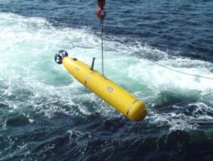
Figure 7. 1. Battlespace Preparation Autonomous Underwater Vehicle (BPAUV) in use during a US Navy exercise. 

Source: Courtesy of Bluefin Robotics Corporation (Copyright belongs to Bluefin and used with permission (https://commons.wikimedia.org/wiki/File:BPAUV-MP_from_HSV-.jpg).

Military applications of UUVs include collecting information, timed strikes, oceanography, payload delivery, mine hunting, network navigation modes, surveillance, anti-submarine operations, reconnaissance, inspection, intelligence gathering, communications enhancement and identification of foreign objects (Department of Defense, 2011) (Department of Defense, 2012).  Figure 7.2 shows the Pluto Plus AUV used for mine identification and destruction by the Norwegian Navy.

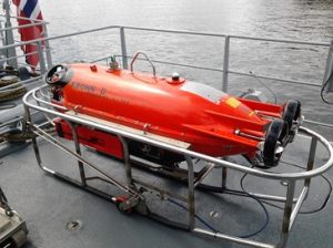
Figure 7.2. Pluto Plus AUV for underwater mine identification and destruction used by the Norwegian mine hunter, KNM Hinnøy. CC BY-SA 3.0.

Source: Created by KEN (https://commons.wikimedia.org/wiki/File:MiniU.jpg)

They are also used for civilian applications such as oil and gas exploration (mapping the sea floor), research vehicles to monitor movements of fish and inspect fauna such as reefs, drug trafficking, air crash investigations, oceanography and many more uses.  UUVs are equipped with sensors such as sonars, thermistors, conductivity probes and magnetometers. Biological sensors include chlorophyll sensors, turbidity sensors and sensors that measure acidity, PH, and the magnitude of dissolved oxygen.

Typically, UUVs lose their GPS signal quickly due to the attenuation of radio waves in water, so they rely on dead reckoning to navigate in water. Acoustic underwater position systems are based on long baseline navigation techniques that can be connected to GPS by allowing the UUV to surface in order to establish its position globally. Owing to the need for surfacing, UUVs are equipped with brush or brush-less motors connected to a gearbox that rotates a propeller that is protected by lip seals and a nozzle. Rechargeable batteries are used and are typically lithium-ion or lithium polymer. Larger UUVs are equipped with fuel cells, but the latest trend is to combine different types of electrical power sources to a supercapacitor.

Role of the Naval Architect

The role of the naval architect is complex and becoming quite broad due to the effects of extreme weather and the minimization of using the earth’s scarce resources (Rydill, 1994).  The naval architect will need to work more closely with natural scientists, such as marine biologists and environmentalists, in order to design vessels that work with nature to minimize the impact on the natural world (Comstock, 1967). The role will continue to work with engineers from other disciplines, project managers and business administrators and we may see the development of new academic programs that blend the principles of naval architecture with business studies that includes the commercial aspects of naval systems such as ‘naval systems architecture’ or ‘marine systems engineering’ (Lewis, 1988) (Taylor, 2006).  In addition to teaching naval architecture from a systems approach, the development of ‘forensic naval architecture’ may provide the safety, reliability and regulatory aspects of naval architecture with the information needed to create naval architects whose design function is clearly guided by knowledge gained from failures using incident/accident reports of submarines that provide valuable data that are contained in codes and standards that allows the design of UUVs that are fit-for-purpose. When designing UUVs, the naval architect must pay special attention to hull shape and to the dynamics of control and its effect on hull shape and associated dimensions.

Naval Architectural Design of UUVs

The design of traditional underwater vehicles (submarines) are based on vessel requirements, weight estimates, initial size, weight and buoyancy balance, arrangements, longitudinal balance, vertical balance and stability, speed and power, propeller, propulsion coefficient, equilibrium polygon, and dynamic stability.  The design of UUVs are very sensitive to weight and buoyancy and the naval architect must balance the cumulative weights with buoyancy of the hull form. A standardized system is used to describe hull structure, propulsion system, electrical system, command and surveillance, auxiliaries, furnishings, armaments, margins and acquisition, and loads (Hughes, 2010).

The use of software in the design of UUVs is prevalent especially when one considers the interdependency of the various aspects of design. Specialized modules of programs are designed to focus on the hull, resistances, loads, and control aspects of the UUV.  The major features of a UUV include the control surface, hull, battery pack, pressure vessel and stiffeners, the battery system, ballasting, controllers, and the payload. Current designs of UUVs have variable hull geometries based on torpedo shapes but some are rectangular shaped that can be hydrodynamically very challenging.

The standard hull envelope for a UUV is axisymmetric having an ellipsoid fore-body, a parallel mid-body and an aft-body shaped like a parabola (Figure 7.3).  This is known at the Jackson hull-form and the diameter of the hull envelope (Eq. 7.1):

                                                               D = L / (L/D)          (7.1)

Where, D is the diameter of the hull envelope and L is the length of the hull.  The length of the fore-body, L_fwd, is a function of the forward hull section length factor, C_fwd, and the diameter of the hull (Eq. 7.2):

                                                    L_fwd = D.C_fwd = C_fwd . (L/(L/D))       (7.2)

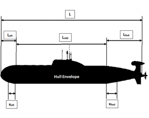
Figure 7.3. Jackson hull-form geometry.

Source: [Adapted from Openclipart Vectors by Pixabay (Public Domain Image)]

Also, the length of the aft-body, L_aft, is a function of the hull-section length factor, C_aft, and hull diameter, D,    (Eq. 7.3):

                                                                      L_aft = D._Caft = C_aft. (L/(L/D))         (7.3)

The parallel mid-body length, L_mid, (Eq.7.4)

                           L_mid=L-(L_fwd L_aft )=L-{(D.C_fwd ) (D.C_aft )}=L[1-((C_fwd C_aft ))/((L/D) )]       (7.4)

The sum of the forward and aft length factors must be less than the length-to-diameter ratio. If it is equal, then the UUV will have no mid-section.  Ellipsoidal forward sections have a radial offset, y_fwd, from the centerline of the full length of the UUV body at a local distance, x_fwd, measured from the aft component of the forward body and the forward hull section curvature factor, n_fwd (Eq. 7.5)

 y_fwd=D/2 [1-(x_fwd/L_fwd )^(n_fwd ) ]^(1/n_fwd )           (7.5)

Paraboloid aft-sections have a radial offset, y_aft, from the centerline of the full length of the UUV body at a local distance, y_fwd, measured from the aft-component of the forward body and the forward hull section curvature factor, n_aft (Eq. 7.6)

                                                          y_aft = D/2 [1-(x_aft/L_aft )^(n_aft ) ]                     (7.6)

The construction of tables of offsets allows one to calculate principal characteristics in accordance with naval architectural practices such as prismatic coefficient (C_prismatic), wetted surface area (S), sectional area, and area of the UUV envelope (V_effective).

The resistance to motion is a function of the basic control surface and its propeller.  The calculated resistance allows the naval architect to select the appropriate battery power for the UUV, so it is important to calculate propulsion resistance.

The total ship resistance, R_total, is composed of a number of collective resistances that are expressed as non-dimensioned coefficients. The total resistance coefficient, C_total, is a function of water density, ρ, the wetted surface area, S, and the velocity of the UUV, (Eq. 7.7)

                                                       C_total = R_total/(1/2 ρSV^2 )            (7.7)

When the UUV is operating near to the air-water surface, the resistance is dominated by wave-making resistance and viscous resistance of the fluid.  The wave-making resistance is a function of the Froude number (Fr) and viscous resistance is a function of the Reynolds’ number (Re).  Froude number is a function of velocity, V, gravitational acceleration, g, and length of the hull, L (Eq. 7.8)

                                                                         Fr=V/√(g.L)                  (7.8)

Viscous resistance is given by Re which is a function of velocity, V, length of the hull, L, and the kinematic viscosity of water, υ, (Eq. 7.9)

                                                                             Re=(L.V)/υ                 (7.9)

The total resistance coefficient, Ctotal, is a function of the Froude number and the Reynolds’ number and is approximated as the sum of the coefficients of wave-making and viscous resistances (Eq. 7.10)

                                                          C_total ≈ C_(wave.) Fr + C_viscous.Re         (7.10)

It is noted that the wave-making resistance is work done by the hull on the surrounding fluid to generate waves.  However, there is no resistance of this kind when the UUV is submerged three diameters from the surface of the air-water boundary.  Therefore, at lower depths, resistance is purely viscous and is composed of frictional and residual resistances (Eq. 7.11)

                                                   C_total = C_viscous =  C_friction+C_residual         (7.11)

Frictional resistance in water is a function of Reynolds’ number (Eq. 7.12)

                                                     C_friction=0.075/(log10. (Re)-2)^2      (7.12)

Equation 7.12 is based on tank towing models and not full-scale models.  It is important to calculate empirical resistances that approximate to a value that is similar to actual conditions of submerged motions.  Therefore, the following models provide an estimation of total resistance of UUVs assuming that the hull form is deeply submerged.

Bottaccini Model:

         C_total=[(S.C_friction)/(A.(L/D)^4 )].[(L/D)^4+1/2 (L/D)^3+6]    (7.13)

The hull form is deeply submerged in a viscous fluid operating at small angles of motion. The maximum cross-sectional area, A, is function of hull diameter, D, such that (Eq. 7.14)

                                                A = (πD^2)/4 = π/4 (L/{L/D} )^2            (7.14)

The coefficient of total resistance is also considered to be a function of the coefficient of frictional resistance, the geometry of the hull and the roughness of the surface of the UUV.  This is incorporated in the Gilmer and Johnson model (Eq. 7.15)

Gilmer and Johnson Model:

          C_total = C_viscous+C_roughness = {C_friction [1+D/2L+3(D/L)^3 ]}+C_roughness      (7.15)

The Jackson Curve-Fit Model is a model that is a function of the non-dimensional hull parameter, K (Eq. 7.16), which is based on the length, L, diameter, D, and wetted area, S, of the UUV

                                                   K = (L/D)-(S/(πD^2 ))        (7.16)

And the coefficient of residual resistance is (Eq. 7.17)

Jackson Curve Fit Model:

                                                          C_residual=0.0008/((L/D)-K)           (7.17)

Another model that accounts for the residual resistance is the Jackson-Hoerner model that is a function of frictional resistance, hull diameter and the length of the aft-body (Eq. 7.18)

Jackson-Hoerner Model:

                                   C_residual=C_fwd {[1.5(D/L_aft )^1.5 ]+[7(D/L_aft )^3 ]}        (7.18)

Eq. 7.18 is used when the aft end of the UUV has a significant wake, or a large effect on the form coefficient owing to the separation of flows.  The shape of the UUV in terms of its prismatic coefficient is described by the Jackson Parallel-Mid Body model (Eq. 7.19)

Jackson Parallel Mid-Body Model:

    C_total={C_fwd (1+[1.5(D/L_aft )^1.5 ]+[7(D/L_aft )^3 ]+[0.002(Cprismatic-0.6)])}+C_aft    (7.19)

And to include the effects of the forward and aft hull section curvature factor of the UUV, the Martz model is used to account for the effect of shape of the UUV (Eq. 7.20)

Martz Model:

          C_total={C_fwd (1+(1/2(L/D) )+[3(D/L)^((7-n_fwd-(1/(2n_aft ))) ) ])}+C_aft     (7.20)

Design algorithms incorporate the resistance models to predict the total bare hull resistance of the UUV (Eq.  7.21)

                                              R(_{hull total})=0.5ρSV^2 [0.2(C_total )]       (7.21)

The appendages that are attached to the control surfaces produce their own contribution to flow resistance of UUVs. The equation accounts for hull geometry (length and diameter) and the wetted surface area, S, (Eq. 7.22)

                                            C_appendages = (L.D)/(1000.S_appendages )        (7.22)

The total appendage resistance is given by Equation 7.23

                              R_appendages=0.5ρSappendages V^2 C_appendages=(ρLDV^2)/2000      (7.23)

For the total control of the UUV, the lateral surface area must be known (Equation 7.24)

                         A(_{control surface}) = 0.028.A(_{control surface hull}) = 8.A(_{control surface lateral area})     (7.24)

The size of all control surfaces is important when specifying the amount of power needed to move the UUV through the fluid and the effective horsepower associated with the UUV is (Eq. 7.25)

                                                             P_effective = V(R_hull-R_appendages )/550     (7.25)

For the set operating velocity, the shaft horsepower is that used to provide the primary propulsion in the direction of travel, thus (Eq. 7.26)

                                                           P_shaft=P_effective/C_propulsion           (7.26)

Once the amount of power is known based on the resistances and the shape and size of the UUV, then an estimate of how many batteries and the type of batteries to be used in the UUV can be calculated.

Control and Dynamics of UUVs in Water

The shape of a UUV has significant effects on hydrodynamic signatures and places limitations on the control surfaces relative to the center of gravity.  The shape can be changed by adding appendages and the positioning of rudders and spaces for hydroplanes, which usually affects the dynamics and control of such vehicles when submersed.  This also changes the amount of power required to provide thrust (MAN Energy Solutions, 2018). The motion in the six degrees-of-freedom is usually referred to as heave, yaw, sway, roll, surge, and pitch (Figure 7.4).

EQUATIONS OF MOTION FOR UUVs

The equations of motion describe the axes that are aligned to UUVs such as longitudinal, vertical, athwartships that allow the UUV to move in three dimensions in hydrospace, the center of which is set by the center of the geometric center of the UUV, or the center of gravity (Mollard, 2013). The following equations describe the equations of motion in accordance with the convention shown in Figure 7.4.

Surge equation:

                                                     mu ̇=X_P+X_U+X_M+X_A        (7.27)

The surge equation describes the mass of the UUV multiplied by its acceleration being equal to the sum of its forces acting in the longitudinal direction, where X_P is the propulsive thrust force, X_U is the hydrodynamic resistance force, X_M is the drag force due to lateral motion and X_A is the hydrodynamic force due to lateral acceleration.

Horizontal plane equations:

                                                      m(v ̇+  rU)=Y_V+Y_V ̇ +Y_R+Y_Control        (7.28)

And

                                                        I_zzr ̇=N_V+N_R+N_{R ̇} +N_Control        (7.29)

Equation 7.28 represents the action of mass of the UUV and its sideways acceleration through the horizontal plane of motion and Equation 7.29 describes the product of rotating inertia about the vertical axis through the center of gravity and its angular acceleration in yaw to the sum of horizontal moments of hydrodynamic forces acting on the hull of the UUV.

Vertical plane equations:

                                             m(w ̇+qU) = Z_W+Z+Z_θ+Z_Control          (7.30)

And

                                             I_yyq ̇=M_W+M_Q+M_θ ̇ +M_Control           (7.31)

Equation 7.30 represents the action of rigid mass of the UUV and its acceleration in the vertical plane of motion to the sum of the hydrodynamic forces acting on the hull and Equation 7.31 describes the product of rotating inertia about the horizontal axis through the center of gravity and its angular acceleration in pitch to the sum of vertical moments of hydrodynamic forces acting on the hull of the UUV, supplemented with a restoring moment due to movements away from the horizontal (Rydill, 1994).

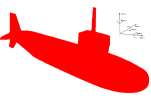
Figure 7.4. Freedom of motion for UUV.

Source: [Adapted from Open Clip art Vectors by Pixabay (Public Domain Image)]

Roll equation:

                                                                      IxxΦ =K_v+K_R+K_Φ          (7.32)

The roll equation (Eq. 7.32) describes the product of rotating inertia about the longitudinal axis and its angular acceleration in roll to the sum of athwartships moments acting on the hull due to hydrodynamic restoring moments owing to movements away from the vertical axis. Control forces are those that account for rigid body forces and those considered control forces owing to motions in vertical, horizontal, and longitudinal directions. Hydrodynamic forces should also be considered as they are considered to be directly proportional to small changes in velocity when UUVs depart from initial straight-line motions.  They are known as derivatives owing to those small changes from the straight-line path of motion (Lewis, 1988).

HYDRODYNAMIC DERIVATIVE FORMS

                                                             Y^’_v= Y_V/(0.5ρUL^2 )       (7.33)

The derivative form is dimensional and as an example, Equation 7.33 is dimensionless owing to its constant characteristic of the UUV’s geometry. In its dimensioned form, hydrodynamic derivatives are dependent on the square of the velocity of the UUV.

STABILITY AND CONTROL IN THE HORIZONTAL PLANE

When the derivative approach is applied to the equations of motion and adapted to include control terms appropriate to the rudder’s deflection to the angle, δ, the linear equations is sway velocity, v, and yaw rate, r, are defined (Eq. 7.34 and 7.35).

Equations in derivative form:

                                                       m(v ̇+rU)=Y_v v+Y_{v ̇} v ̇+Y_rr+Y_δ δ             (7.34)

And

                                                           I_zzr ̇= N_vv+N_rr+N_r r ̇+N_δδ                    (7.35)

Equations 7.34 and 7.35 show two unknowns, v, and r (sway velocity and yaw rate), as a function of the control term, δ. For dynamic stability, it is assumed that the UUV is moving in water on a straight path with no control input (δ=0).

Dynamic stability:

                                                           v ̇(m-Y_v ̇ )=Y_v v + r(Y_r-mU)           (7.36)

And

                                                        r ̇(I_zz-N_r ̇ ) = N_v v+N_r r                    (7.37)

The equations shown here can be solved using transformations into a single linear equation for either v and r. The general form of equations can be expressed in real or imaginary terms and tend to indicate whether the UUV is stable or unstable along its path of motion. The control effectiveness of the rudder can be understood by analyzing steering motions as function of rudder force (Lewis, 1988).

Steering motions:

                                                       Y_vv+(Y_r-mU)r+Y_δ δ=0              (7.38)

And

                                                           N_vv+N_r r+N_δ δ=0                    (7.39)

And

                                                r/δ = Y_δ/((Y_r-mU) ) (x_v-x_δ)/(x_r-x_v )         (7.40)

Here, it is understood that all terms associated with derivatives are omitted and we are left with constant velocity terms.  Equations 7.38 and 7.39 can be solved to give a steady state turn, r, as a function of rudder deflection, δ, (Equation 7.40).  The equation tells us that the rudder should be placed aft of the body as far as possible in order to gain the best control of the UUV due to the sway of the hydrodynamic forces on the hull (Comstock, 1967).

STABILITY AND CONTROL IN THE VERTICAL PLANE

For vertical control of the UUV at velocity, w, and pitch angle, θ, the rate of change of pitch angle is needed. It is also required to know two sets of control surfaces with two deflection angles of δf on the forward and aft hydroplanes (Eqs. 7.41 – 7.43).

Equations in derivative form:

                                                     m(w ̇+rU) = Z_w w+Z_q q+Z_δfδf+Zδa δ_a           (7.41)

And

                                               I_zzq ̇=M_w w+M_qq+M_θ θ+M_δfδ_f+M_δa δ_a              (7.42)

                                                             M_θ=W.(BG) ̅                                             (7.43)

The hydrostatic restoring moment in Equation 7.42 is associated with the pitch angle that indicates a preferential motion in the vertical plane. The UUV can be considered moving along a straight line with no input from the rudder (δf and δa = 0), which leads us to define dynamic stability.

Dynamic stability:

                                                                (w ̇-qU)=Z_ww+Z_qq             (7.44)

And

                                                              I_yyq ̇= M_ww+ M_wq  +W.(BG.θ) ̅          (7.45)

Equations 7.44 and 7.45 are simplified forms of the equations of motion and have three roots that will be dependent on the speed of the UUV.  When the control surfaces are operating in response to rudder motions, Equations 7.46 – 7.50 apply.  The combined effects of control forces are shown in Equation 7.46.

Motion control with surfaces operating:

                                                           Z_αα+Z_δcδ_c=0                 (7.46)

And

                                                          M_αα+M_θθ+M_δcδ_c=0       (7.47)

Equation 7.46 allows us to derive the vertical velocity as the function of control surface angles of deflection (Eq. 7.48).

                                                         α = -(Z_δcδc)/Z_α                 (7.48)

Here (Eq. 7.48), the vertical velocity is related to the control force and the hydrodynamic resistance of the UUV in vertical and horizontal directions.  Using the solution from Equation 7.46 to feed into Equation 7.47, the pitch angle is a function of angles of deflection of the control surfaces (Equation 7.49):

                                                        θ = (Z_δc δ_c (xα-xc ))/M_θ               (7.49)

Where x_c=(M_δc)/Z_δc and x_a=M_α/z_α                                                   (7.50)

Equations shown in 7.50 are the effective locations of control and heave forces, respectively.  The equations shown in this section are used to control pitch and plane setting in UUVs and are critical when coupled with the shape of the hull to reduce flow signatures.  It is noted that hull form and shape and appendages are critical aspects of control dynamics, so much analysis is performed by the naval architect to perfect the design of UUVs prior to construction (American Bureau of Shipping, 2019).

Structural Integrity

Once the shape, form and control aspect of the UUV is accepted, the structural integrity of the UUV is calculated by understanding the structure of materials and how they can withstand hyperbaric pressures at known depths (American Bureau of Shipping, 2019).

External hydrostatic pressures are calculated for each control surface and materials are selected by understanding the three primary failure modes (Lewis, 1988):

• axisymmetric yielding of the shell between stiffening frames characterized by elastic-plastic collapse (concertina effect);
• shell buckling between stiffening frames characterized by buckling forming inward and outward bulges of the shell; and
• Instability that occurs between bulkheads and frames and results in elastic buckling of the frame-shell of the hull.

Knowledge of materials are required to select the best material for the UUV shell. This means that design factors such as buckling pressure, yielding pressure at the frame, yielding pressure at mid-bay, general instability, frame instability buckling pressure, frame hoop stress and total frame hoop stress for the structure need to be calculated (Hughes, 2010). The current ABS Rules governing the design of UUVs considers the following structural design factors:

• Stiffener strength;
• Buckling strength;
• Longitudinal frame strength;
• Inner stiffener strength;
• Local stiffener flange buckling strength;
• Local stiffener web buckling strength; and
• Combined stiffener and shell moment of inertia.

Stiffener and web spacings are calculated to avoid the three modes of failure based on the strength properties of the material(s) selected for the UUV shell (American Bureau of Shipping, 2019).

Discussion / Conclusions

The detailed information generated by the naval architect to design the hull shell and its appendages according to its mission in the water is used to allow the architect calculate how much battery power is needed for the UUV (Rydill, 1994). The selection is based on the propulsive and static loads needed to move the UUV and its apparent and real volume.  Batteries need to be carried on board, so the size related to their energy density is critical.  Typically, lithium-ion batteries are used because they have such a large energy density (~1300 HP.min/ft3), whereas lead-acid batteries are typically not used because of their low energy density (~160 HP.min/ft3).  It should be noted that current battery technology severely limits the naval architect who is responsible for the design of UUVs.  Advances in the field of fuel cells and associated systems such as supercapacitors are long awaited.

Questions

1. What is a naval architect and how does it affect the design of UUVs?
2. Describe the shape of a UUV and how its shape can affect how it operates.
3. Explain the differences in the flow resistance models and how they are incorporated into the design procedures for UUVs.

References

American Bureau of Shipping. (2019). ABS Rules for Building and Classifying Underwater Vehicles, Systems and Hyperbaric Facilities. Houston, Texas: American Bureau of Shipping.

Button, R. W. (2009). A Survey of Missions for Unmanned Undersea Vehicles. Santa Monica, California, USA: RAND Corporation.

Comstock, J. P. (1967). Principles of Naval Architecture. New York, USA: Society of Naval Architects and Marine Engineers.

Department of Defense. (2011). Unmanned Systems Integration Roadmap: 2011 – 2036. Washington DC, USA: US Government.

Department of Defense. (2012). Sustaining US Global Leadership: Priorities for the 21st Century Defense. Washington DC, USA: US Government.

Department of the Navy. (2004). The Nay Unmanned Undersea Vehicle Master Plan. Washington DC, USA: US Government.

Hughes, O. F. (2010). Ship Structural Analysis and Design. New York, USA: Society of Naval Architects and Marine Engineers.

Lewis, E. V. (1988). Principles of Naval Architecture: Volumes I, II and III. New York, USA: Society of Naval Architects and Marine Engineers.

MAN Energy Solutions. (2018). Basics of Ship Propulsion. Berlin, Germany: MAN.

Mollard, A. F. (2013). Ship Resistance and Propulsion. Cambridge, UK: Cambridge University Press.

Pengelly, E. L. (1956). Theoretical Naval Architecture. London: Longmans.

Rydill, R. B. (1994). Concepts in Submarine Design. Cambridge, UK: Cambridge University Press.

Taylor, D. A. (2006). Merchant Ship Naval Architecture. London, UK: The Institute of Marine Engineering, Science and Technology.