5 Infinite Impulse Response (IIR) Filter Design
IIR Filters
The next type of filter we will be designing are called Infinite Impulse Response (IIR) filter. These filters will use a feedback of the output in order to generate the next sample, causing a infinite ripple in the output. These filters are primarily going to be built by translating the analog filters described in Appendix B, into discrete forms.
Section A) Feedback Discrete Systems
Unlike the FIR filters of chapter 4, the filters in this section will employ feedback of previous outputs to generate the next output. This causes the output of the system to ripple for a long time, hence the name of Infinite Impulse Response (IIR) filters. Another way these filters are described as Pole-Zero (PZ) filters, since the feedback creates poles in the z-transform transfer function.
Section A.1) Impulse Response
We have touched on these types of filters in chapter 3, when we were developing the z-transform. The best example would be the simple case of a first order system
[latex]y(n) = x(n) + a y(n-1)[/latex] (5.1)
The signal flow diagram of which is
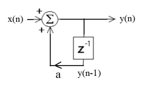
Figure 5.1 First Order Signal Flow Diagram.
In order to build an image of these systems and their response, consider the output y(n) to an input that is an impulse
[latex]\delta(n) = \{_{0\text{ otherwise } }^{1 \text{ for n = 0}}[/latex]
Since the input is zero for all n < 0, the output is also 0.
[latex]y(n) = 0 \text{ for n } \lt 0[/latex]
At time 0, the input is a one and then
[latex]y(0) = x(0) + a y(-1) = 1 + a 0 = 1[/latex]
[latex]y(1) = a*y(0) + x(1) = a[/latex]
[latex]y(2) = a*y(1) + x(1) = a^2[/latex]
[latex]y(3) = a*y(2) = a^3[/latex]
…
[latex]y(n) = a^n[/latex] (5.2)
As we can see from this result, the output of such a system from an impulse input is and infinite signal. Hence the name of Infinite Impulse Response (IIR) filter. Although interesting, the impulse response of a discrete system such as this is not directly used to design or interpret an IIR filter. Rather we need to look at the frequency response, which is the primary character we will be designing for. A quick review of Section 3, would be helpful in understanding the follow developments.
Section A.2) Frequency Response
As stated in the previous section, chapter 3 addressed the Frequency Response (FR) of discrete systems. And when we were building FIR filters we were able to first simply write out the FR for a generic set of coefficients. Then solve these for a given FR. In the case of IIR filters, we will need to work this from a different angle. Here we will need to look at how the pole locations affect the FR and how we can develop specific patterns to create the FR that we want.
If we look back at chapter 3, we can see the FR of a system with feedback has poles which pull the [latex]H( e^{j \omega} )[/latex] towards infinity. This effect will mean we will need a distinct pattern of poles to get the desired FR. This phenomena is also seen in the design of an analog filter. As shown here, the Butterworth filter has a set of poles that form a circle near the imaginary or jw axis in the analog s-plane. ( A reading of Appendix B might be in order at this time. )
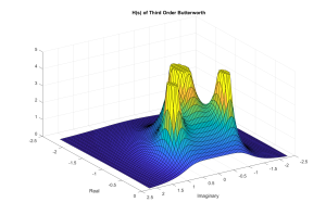
Figure 5.2 Magnitude of Third-Order Butterworth H(a+jw)
Close observation of the previous circle of poles, we can see that the pattern of three poles work together to create a very smooth low-pass filter along the imaginary (jw) axis. In the case of a discrete system, we will see that the pattern is not easily defined in the z-plane. Rather we will work by taking an analog filter and translating to a discrete implementation.
Section B) Bi-Linear Transform
If you have reviewed the analog filters in Appendix B, you should note that the classic design of analog filters involves the transforming (mapping) of low-pass, high-pass and band-pass filters into a normalized low-pass filter. A canonical or standardized filter is then matched to that normalized low-pass, which is then translated back to the desired form. With the IIR filter we will need to find a mapping that takes our digital frequency response and translates it into an analog filter specification. Basically to map between the z and s planes.
We actually had a mapping when we developed the z transform and it was [latex]z = e^{sT}[/latex], however this is not a one-to-one mapping. Also if we take this equation and solve for s, we get [latex]s = \frac{1}{T} ln(z)[/latex], which if we substitute it into H(s), does not produce a valid H(z). Another approach is to use the Bi-Linear (BL) transformation given by
[latex]s = \frac{z-1}{z+1}[/latex] or [latex]z = \frac{1+s}{1-s}[/latex] (5.3)
The BL transformation is a one-to-one transformation and produces a valid H(z). As a way to visualize this transformation, consider the following points.
If [latex]s = 0 \Rightarrow z = 1[/latex]
and [latex]s = +j \Rightarrow z = \frac{1+j}{1-j} = \frac{(1+j)(1+j)}{(1-j)(1+j)} = \frac{1+2j-1}{2} = +j[/latex]
Similarly [latex]s = -j \Rightarrow z = -j[/latex]
If we let [latex]s \to +\infty \Rightarrow z \to \frac{1+\infty}{1-\infty} \to \frac{+\infty}{-\infty} = -1[/latex]
Similarly [latex]s \to -\infty \Rightarrow z \to \frac{1-\infty}{1+\infty} \to \frac{-\infty}{+\infty} = -1[/latex]
A visual representation of this mapping is shown in Figure 5.3, emphasizing the previous five points. An important point is that the [latex]j \omega[/latex] axis maps onto the unit circle. Both of which represents the FR of the systems.
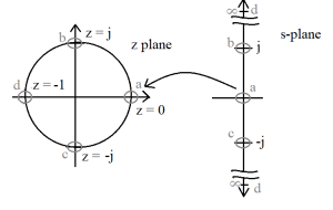 Figure 5.3 Conformal Mapping for BL Transformation
Figure 5.4 shows the mapping in a slightly different form, showing the mapping of points along the frequency axis.
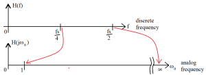
Figure 5.4 BL Mapping Across Frequency Axes.
With this in mind, let’s walk through a process, by which we could create a discreet feedback system with a given FR.
Section B.1 Bi-Linear Filter Design Procedure
The following steps are how most systems design a discrete-feedback or IIR filter to have a given FR.
Design Procedure
1) Set the sampling frequency, [latex]f_s[/latex] and define the discrete frequency response for the range ([latex]\omega = 0 \to pi[/latex], or [latex]f = 0 \to \frac{f_s}{2}[/latex]).
An example would be to assume a sampling rate of 10 KHz and design a high-pass filter as shown here.
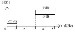
Do note that the range is from 0 to [latex]\frac{f_s}{2}[/latex] = 5 kHz which is all that is needed, since all other frequencies are reflections of the response at these frequencies.
2) The critical frequencies should now be translated to the matching analog frequencies. This translation starts by equating the analog and digital frequencies as shown here.
[latex]s = j \omega_a = {\frac{z - 1}{z+1}}|_{z = e^{j \omega T}} = \frac{e^{j \omega T} - 1} {e^{j \omega T} + 1 }[/latex] (5.4)
where [latex]\omega_a[/latex] is the analog radial frequency ([latex]0 \to \infty[/latex]) and [latex]\omega[/latex] is the digital radial frequency ([latex]0 \to \pi[/latex])
[latex]j \omega_a = \frac{e^{j \omega \frac{T}{2}} (e^{j \omega \frac{T}{2}} - e^{-j \omega \frac{T}{2}})}{e^{j \omega \frac{T}{2}} (e^{j \omega \frac{T}{2}} + e^{-j \omega \frac{T}{2}})} = \frac{2 j sin( \omega \frac{T}{2} )}{ cos( \omega \frac{T}{2} ) } = j tan( \omega \frac{T}{2} )[/latex]
Rarely does anyone use radial frequencies, thus we need to translate to plain frequencies using
[latex]f_s = \frac{1}{T}[/latex] and $latex$ \omega = 2 \pi f$
Resulting in the translation
[latex]j \omega_a = j tan( \frac{\pi f }{f_s} ) [/latex] (5.4)
This equation matches with the frequency mapping from the previous section. With f = 0 [latex]\to \omega = 0[/latex] and f = [latex]\frac{f_s}{2} \to \omega = \infty[/latex].
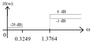
For the example we are working through the critical frequencies are f = 0, 1 kHz, 3 kHz and 5 kHz. Using the (5.4) we have [latex]\omega_a = 0, tan( \frac{\pi}{10} ) \simeq 0.3249, tan( \frac{3 \pi}{10}) \simeq 1.3764[/latex], and $latex\infty$
3a) Using the process described in Appendix B, design an analog filter that matches this spec. The first step is to translate this high-pass filter into a Normalized Low Pass (NLP) filter via [latex]\hat{s} = \frac{wp}{s}[/latex], where wp = 1.3764. This translates the design into
![]()
Note that the upper cutoff (1.3764) has translated to one, while the lower cutoff (0.3249) moves up to 4.236.
3b) Find canonical form that matches this NLP form. The simplest form is the Butterworth filter, where the order of the filter (n) can be computed by the dB per decade or
[latex]-20 n = \frac{20 log(|H(\omega_s)|}{log(\omega_s)} = \frac{-20}{log(4.236)} = - 31.9[/latex]
Rounding up we have n = 2, and the second order Butterworth filter is relatively simple as
[latex]\hat H(s) = \frac{1}{s^2 + \sqrt{2} s + 1}[/latex]
3c) We can now translate this design back to the original frequencies via [latex]\hat s = \frac{1.3764}{s}[/latex], which looks like
[latex]H(s) = \hat H( \hat s ) |_{\hat s = \frac{1.3764}{s}} = \frac{1}{(\frac{1.3764}{s})^2 + \frac{ 1.3764 \sqrt{2}}{s} + 1}[/latex]
[latex]H(s) = \frac{s^2}{s^2 + 1.9465 s + 1.8944}[/latex]
4) We are now ready to create the z-transform transfer function that will define the discrete system. The translation uses the original definition of the BL transform. Which looks like
[latex]H(z) = H(s) |_{s = \frac{z-1}{z+1}} = \frac{\frac{(z-1)^2}{(z+1)^2}}{\frac{(z-1)^2}{(z+1)^2} + 1.9465 \frac{(z-1)}{(z+1)} + 1.8944}[/latex]
multiplying top and bottom by [latex](z+1)^2[/latex] we have
[latex]H(z) = \frac{z^2 - 2 z + 1}{4.8409 z^2 + 1.788 z + 0.9479}[/latex]
To convert this into a difference equation, we begin my multiplying the top and bottom by 0.20657 and z-2 to give
[latex]H(z) = \frac{0.20657 - 0.4131 z^{-1} + 0.20657 z^{-2}}{1 + 0.36957 z^{-1} + 0.1958 z^{-2}}[/latex]
As a check on the FR, we will factor the numerator into +1 ( zeros ) and the denominator into -0.18476 + j 0.402092 (poles). Visually these look like
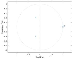
Which indicates a high-pass filter (zeros at 1, f = 0, and poles over closer to -1).
5) Implementation
This transfer function represents the difference equation
[latex]y(n) = -0.36957 y(n-1) - 0.1958 y(n-2) + 0.20657 x(n) -0.4131 x(n-1) + 0.20657 x(n-2)[/latex]
Or the following signal flow graph.
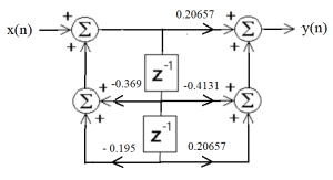
Note this unit is the basic building block for most IIR digital filters. The next section will show how these filters can be developed with the MATLAB signal processing toolbox.
Section C) MATLAB Implementations
The software environment of MATLAB has a collection of functions that allow the user to create filters without having to go through these calculations by hand.
I will start with the basic call to build the filter we worked through in the previous section. As was described in the previous section, the order of the filter we will need to match the specifications, is important. The order can be found using the MATLAB command “buttord”, which will need the passband-corner and the stopband-corner frequencies as well as the passband attenuation tolerance and the stopband attenuation. The call looks something like
n = buttord( 3/5, 1/5, -3, -20 );
The four arguments that are used in command are
- The passband corner frequency (3 k) divided by [latex]\frac{f_s}{2}[/latex] (5 k).
- The stopband corner frequency (1 k) divided by [latex]\frac{f_s}{2}[/latex] (5 k).
- The passband gain tolerance (-3 dB).
- The stopband attenuation (-20 dB).
Included here is the original specification of the filter, in the digital frequency domain.
Once we know the order needed we can generate the filter in question using the butter command, shown here
[B,A] = butter(n,3/5,’high’)
B =
0.2066 -0.4131 0.2066
A =
1.0000 0.3695 0.1958
The arguments are
- The order of the filter ( 2 )
- The passband cutoff frequency ( 3k / 5k )
- Type of filter ( Optional, if non-given a low-pass filter is assumed )
and the outputs are
- The numerator of H(z) for the filter
- The denominator of H(z)
It should be noted that the numbers generated by the command “butter” as the coefficients, match those computed previously.
Much like the analog filters, IIR filters can be generated using the Butterworth or Chebyshev configuration and MATLAB supports these types, with similar commands. The pdf, that is linked in here, demonstrates how these two types of filters can be created in MATLAB.
As alluded to in the previous posting, high-order filters cannot be accurately represented by polynomials. In the next posting, it will be shown to be a case of round off error. Fortunately, MATLAB has an approach that represents the filters in the form of poles and zeros, which represents the filter perfectly.
In order to complete the process, an example of how filters can be implemented in the c language is included here. Do note that the filters designed are used to filter a sweeping cosine, or what some call a chirp, in order to visualize the frequency response of the filters.
