6 Discrete Fourier Transform
The Fourier Transform has been employed from the beginning of this text, however it is commonly used in the continuous “analog” domain. When we are dealing with discrete data however, some of the details are different. We will start with the basic definitions of what is known as the Discrete Fourier Transform (DFT), establishing some of its basic properties. Moving on we will do a couple application of the DFT, such as the filtering of data and the analysis of data. Another important part of will be the computation of the DFT using what is known as the Fast Fourier Transform (FFT).
Section A) DFT Basics
The DFT is actually a process of approximating a function by a weighted sum of basis functions. The basis function that has proven to be the most effective, not just in the discrete domain but in all forms, is the complex exponential. If we are analyzing a signal that is N points long, this basis function looks like
[latex]b_k (n) = e^{j \frac{2 \pi}{N} k * n }[/latex]
An important feature of the basis function is that it is N periodic. This can be seen by evaluating at (n + m * N) .
[latex]b_k (n+m*N) = e^{j \frac{2 \pi}{N} k (n+m*N) }[/latex]
Factoring [latex]e^{j \frac{2 \pi}{N} k (n+m*N) }[/latex] into
[latex]b_k (n+m*N) = e^{j \frac{2 \pi}{N} k (n) } e^{j \frac{2 \pi}{N} k (m*N) }[/latex]
Cancelling out the N terms
[latex]b_k (n+m*N) = e^{j \frac{2 \pi}{N} k *n } e^{j {2 \pi} * k * m }[/latex]
And finally noting that [latex]e^{j {2 \pi} * k * m } = 1[/latex] for all k and m
[latex]b_k (n+m*N) = e^{j \frac{2 \pi}{N} k *n } = b_k (n)[/latex]
Showing that [latex]b_k (n)[/latex] repeats ever N samples.
We will now look at how this basis function is used to approximate a signal.
Section A.1) Approximation of x(n) via the DFT.
We can then approximate a function x(n) as a weighted sum of these basis functions.
[latex]\hat x(n) = \sum_{k=0}^ {N-1} X(k) b_k(n)[/latex]
or
[latex]\hat x(n) = \sum_{k=0}^{N-1} X(k) e^{j \frac{2 \pi}{N} k * n}[/latex]
To solve for the term X(k), which represents the weighting of each function bk(n) we will work to minimize the Least Squared Error. The first step is to write the error expression as
[latex]\epsilon = \sum_{n=0}^{N-1} | x(n) - \hat x(n) |^2[/latex]
assuming x(n) and [latex]\hat x(n)[/latex] could be complex we would have
[latex]\epsilon = \sum_{n=0}^{N-1} ( x(n) - \hat x(n) ) (x(n) - \hat x(n) )^*[/latex]
Substituting in the definition of [latex]\hat x(n)[/latex] we have
[latex]\epsilon = \sum_{n=0}^{N-1} ( x(n) - \sum_{k=0}^{N-1} X(k) e^{j \frac{2 \pi}{N} k n} ) (x^*(n) - \sum_{m=0}^{N-1} X^*(m) e^{-j \frac{2 \pi}{N} m n} )[/latex]
Completing the product of the two equations under the sum and then distributing the sum we have
[latex]\epsilon = \sum_{n=0}^{N-1} | x(n) |^2 - \sum_{k=0}^{N-1} X(k) \sum_{n=0}^{N-1} x^*(n) e^{-j \frac{2 \pi}{N} k n} - \sum_{m=0}^{N-1} X^*(m) \sum_{n=0}^{N-1} x(n) e^{j \frac{2 \pi}{N} m n} + \sum_{k=0}^{N-1} X(k) \sum_{m=0}^{N-1} X^*(m) \sum_{n=0}^{N-1} e^{j \frac{2 \pi}{N} (k-m) n} )[/latex]
Now this is rather long and tedious, but if we look at the last sum, it can be shown to be a geometric series which has a solution of
[latex]\sum_{n=0}^{N-1} e^{j \frac{2 \pi}{N} (k-m) n} = \frac{1-e^{j(k-m) \frac{2 \pi}{N} N}} {1-e^{j(k-m) \frac{2 \pi}{N}}}[/latex]
[latex]\sum_{n=0}^{N-1} e^{j \frac{2 \pi}{N} (k-m) n} = \frac{1-e^{j{2 \pi} (k-m)}} {1-e^{j \frac{2 \pi}{N}(k-m) }}[/latex]
[latex]\sum_{n=0}^{N-1} e^{j \frac{2 \pi}{N} (k-m) n} = \frac{1-(1^{ (k-m)})} {1-e^{j \frac{2 \pi}{N}(k-m) }}[/latex]
if k = m
[latex]\sum_{n=0}^{N-1} e^{j \frac{2 \pi}{N} 0 n} =\sum_{n=0}^{N-1} 1 = N [/latex]
Otherwise we have
[latex]\sum_{n=0}^{N-1} e^{j \frac{2 \pi}{N} (k-m) n} = \frac{1-1} {1-e^{j \frac{2 \pi}{N}(k-m) }} = \frac{0} {1-e^{j \frac{2 \pi}{N}(k-m) }} = 0[/latex]
This is commonly called the orthogonality property. Thus the two sums at the end of the previous equation collapse to one, since the sum under them is zero, except when k = m.
[latex]\epsilon = \sum_{n=0}^{N-1} | x(n) |^2 - \sum_{k=0}^{N-1} X(k) \sum_{n=0}^{N-1} x^*(n) e^{-j \frac{2 \pi}{N} k n} - \sum_{m=0}^{N-1} X^*(m) \sum_{n=0}^{N-1} x(n) e^{j \frac{2 \pi}{N} m n} + \sum_{k=0}^{N-1} X(k) X^*(k) N [/latex]
We now take the partial derivative of the error [latex]\epsilon[/latex] with respect to one of the weights X(L).
[latex]\frac{\partial{ \epsilon }}{\partial{X(L)} } = 0 - \sum_{n=0}^{N-1} x(n) e^{-j\frac{2 \pi}{N}L n} - \sum_{n=0}^{N-1} x^*(n) e^{j\frac{2 \pi}{N}L n} + N X^*(L) + N X(L) = 0[/latex]
Note that the first sum is not a function of X(L) so its derivative is zero, and the next to sums disappear except for the case of the sum index equal to L. The last sum is only true when k = L and is then separated into its two parts. It is sufficient to recognize that the sum
[latex]X(L) = \frac{1}{N} \sum_{n=0}^{N-1} x(n) e^{-j \frac{2 \pi}{N} L n}[/latex]
is a solution to partial derivative equation above.
Returning to the original definition we have an approximation of x(m) as
[latex]\hat x(m) = \frac{1}{N} \sum_{k=0}^{N-1} X(k) e^{j \frac{2 \pi}{N}k m}[/latex]
Substituting in the solution to our derivation above we have
[latex]\hat x(m) = \frac{1}{N} \sum_{k=0}^{N-1} \sum_{n=0}^{N-1} x(n) e^{-j \frac{2 \pi}{N} m n} e^{j \frac{2 \pi}{N} m k}[/latex]
Reordering the finite sums, we have
[latex]\hat x(m) = \frac{1}{N} \sum_{n=0}^{N-1} x(n) \sum_{k=0}^{N-1} e^{-j \frac{2 \pi}{N} k (m-n)} [/latex]
Note that the sum on the right hand side of the previous equation is the orthogonality property and is equal to N if and only if m = n. Thus
[latex]\hat x(m) = \frac{1}{N} x(m) N = x(m) [/latex]
This leads us to the final point, in that we have a DFT pair of
[latex]X(m) = \sum_{k=0}^{N-1} x(k) e^{-j \frac{2 \pi}{N} m k}[/latex]
[latex]x(n) = \frac{1}{N} \sum_{k=0}^{N-1} X(k) e^{j \frac{2 \pi}{N}k n}[/latex]
The [latex]\frac{1}{N}[/latex] is moved to the inverse strictly by convention. And we need to be aware that the transform from x to X, uses the conjugate of the basis function ( [latex]e^{-j \frac{2 \pi}{N} m k}[/latex] ) and the inverse transform uses the basis function ( [latex]e^{j \frac{2 \pi}{N} m k}[/latex] ) .
Section A.2) Hidden Assumptions in the DFT.
One of the most important “hidden” assumptions about the DFT is that it assumes the sequence that we are analyzing is periodic with a period of N. The term N is the number of points we have been given in the sequence. This periodicity results from the periodicity of the basis function, [latex]e^{j \frac{2 \pi}{N}k * n}[/latex], which was shown in the introduction to this chapter. Consider the inverse transform sum from earlier, and evaluate the output at n+m*N
[latex]x(n+m*N) = \frac{1}{N} \sum_{k=0}^{N-1} X(k) e^{j \frac{2 \pi}{N}k (n+m*N)}[/latex]
Factoring the term [latex]e^{j \frac{2 \pi}{N} k (n+m*N) }[/latex] into [latex]e^{j \frac{2 \pi}{N} k n} e^{j \frac{2 \pi}{N} m*dN }[/latex] and noting that the N’s cancel in the second term we have [latex]e^{j \frac{2 \pi}{N} k n} e^{j 2 \pi m }[/latex] and [latex]e^{j 2 \pi m } = 1[/latex] for all m’s integers, thus
[latex]x(n+m*N) = \frac{1}{N} \sum_{k=0}^{N-1} X(k) e^{j \frac{2 \pi}{N}k n} = x(n)[/latex]
This property / assumption will affect many of the algorithms we will use the DFT for, so please keep it in mind.
Section B) Properties of the DFT.
Again we start with the DFT pair.
[latex]X(m) = \sum_{k=0}^{N-1} x(k) e^{-j \frac{2 \pi}{N} m k} = DFT"{" x(n) "}"[/latex]
[latex]x(n) = \frac{1}{N} \sum_{k=0}^{N-1} X(k) e^{j \frac{2 \pi}{N}k n} = IDFT"{" X(k) "}"[/latex]
Then we will start with some basic properties of the DFT
1) Linearity
DFT{ a x(n) + b y(n) } = a DFT{ x(n) } + b DFT{ y(n) }
The proof of this is rather simple, simply insert a x(n) + b y(n) into the definition of DFT, and then distribute the sum.
DFT{ a x(n) + b y(n) } [latex]= \sum_{k=0}^{N-1} ( a*x(n) + b*y(n) ) e^{j \frac{2 \pi}{N} k * n}[/latex]
DFT{ a x(n) + b y(n) } [latex]=( a* \sum_{k=0}^{N-1} x(n) e^{j \frac{2 \pi}{N} k * n} + b*\sum_{k=0}^{N-1}y(n) e^{j \frac{2 \pi}{N} k * n})[/latex]
DFT{ a x(n) + b y(n) } [latex]=( a* X(k) + b*Y(k) )[/latex]
2) Time and phase shifts
DFT{ x(n – i) } => X(k) [latex]e^{-j \frac{2 \pi}{N} k i }[/latex]
Again the proof is rather simple and straight forward and is not repeated here.
3) The DFT of a signal is Hermitian or has a Complex Conjugate Symmetry about its mid-point.
This is similar to the property of continuous Fourier Transforms (FT) where the real part of the FT is even and the imaginary part is odd. ( real( X(f) ) = real( X(-f) ) and imaginary( X(f) ) = – imaginary( X(-f) ) )
For the DFT, let x(n), 0 < n < N be a real sequence, then
X*(k) = X(N-k) for 0 < k < N
Proof:
[latex]X(N-k) = \sum_{n=0}^{N-1} x(n) e^{-j \frac{2 \pi}{N} n (N-k) }[/latex]
Again we factor out the N and have
[latex]X(N-k) = \sum_{n=0}^{N-1} x(n) e^{j \frac{2 \pi}{N} n k } e^{-j \frac{2 \pi}{N} N n }[/latex]
Since [latex]e^{-j \frac{2 \pi}{N} N n } = e^{-j {2 \pi} n } = 1^n[/latex], we have
[latex]X(N-k) = \sum_{n=0}^{N-1} x(n) e^{j \frac{2 \pi}{N} n k } = X^*(k)[/latex]
Do note that the sign changed on the [latex]e^{j \frac{2 \pi}{N} n k }[/latex] due to the -k in X(N-k).
The next figure is intended to show the relationship in a graphical fashion.
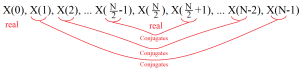
Figure 6-1. Hermitian Symmetry Displayed.
This symmetry will be vitally important when developing filtering employing the DFT.
4) If x(n) is real valued ( like most of the signals we deal with ) then X(0) is real valued
[latex]X(0) = \sum_{k=0}^{N-1} x(k) e^{-j \frac{2 \pi}{N} 0 k} = \sum_{k=0}^{N-1} x(k) 1 = \sum_{k=0}^{N-1} x(k)[/latex] which is thus real valued.
Also if N is even,
[latex]X(\frac{N}{2}) = \sum_{k=0}^{N-1} x(k) e^{-j \frac{2 \pi}{N} \frac{N}{2} k} = \sum_{k=0}^{N-1} x(k) e^{-j \pi k} = \sum_{k=0}^{N-1} x(k) (-1)^k[/latex]
which is again real valued.
5) X(k) is periodic as well
[latex]X(k) = X(N+k)[/latex]
This can be proven by writing out the definition
[latex]X(N+k) = \sum_{n=0}^{N-1} x(n) e^{-j \frac{2 \pi}{N} (N+k) n}[/latex]
Factoring out the N in the exponent, we have
[latex]X(N+k) = \sum_{n=0}^{N-1} x(n) e^{-j \frac{2 \pi}{N} k n} e^{-j \frac{2 \pi}{N} N n}[/latex]
Cancelling out the N, in the second exponent and we have
[latex]X(N+k) = \sum_{n=0}^{N-1} x(n) e^{-j \frac{2 \pi}{N} k n} e^{-j 2 \pi n}[/latex]
Then noting that [latex]e^{-j 2 \pi n} = 1^n = 1[/latex] we have
[latex]X(N+k) = \sum_{n=0}^{N-1} x(n) e^{-j \frac{2 \pi}{N} k n} = X(k) [/latex]
The properties listed here are just a small subset of the various properties that can be developed for the DFT. However these are the ones that commonly come up when applying the DFT to filtering or data analysis.
In order to exemplify these properties, we will look at the results of computing the DFT in MATLAB. Then identify how these properties affect the results. Consider the following MATLAB code and the resulting plot.
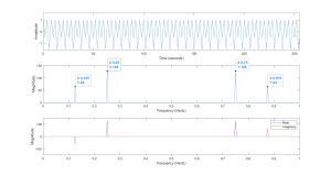
Figure 6.2 Display of DFT, Input, Magnitude and Real-Imaginary Components.
In the previous code and plot, we used two basic components of a cosine at 0.25 Hz and a sine at 0.125 Hz. This gives a waveform with a clean transform, but that is needed so that we can easily interpret the results. As we can see in the plot of the magnitude of the transform, a spike appear at the frequency of each wave, however the magnitudes are affected by the length of the sequence. It should be noted that the larger magnitude cosine wave has a height of 128 or N/2. There are a variety of ways to interpret this, but recall that when defining the DFT pair (forward and reverse transforms) it was noted that a divide by N was needed and arbitrarily placed on the reverse transform.
Another important feature is that each wave produces two pulses in the transform. Due to the way that the DFT is defined, the second pulse from each wave actually represents the negative frequency for each. In the case of the cosine these are at 0.25 and 0.75, which is fs – fo = 1 – 0.25 = 0.75 . Also important to note is that the sine appears in the transform at 0.125 and 0.875, which is ( 1 – 0.125 ).
Just looking at the magnitude plot, an important piece of information is lost in that the cosine and sine look the same. In the last plot the real and imaginary parts of the transform are plotted separately, showing how cosine/sine affect the transform. The cosine appears in the real portion (blue trace) of the transform as pulses at 0.25 and 0.75, while the sine appears in the imaginary portion (red trace) of the transform at 0.125 and 0.875. In the magnitude plot this was lost, but could be represented by a phase plot. However the phase becomes rather “random” away from the components and is very hard to read. The value of the phase at the components is telling, with the phase at 0.25 and 0.75 (cosine) being 0 degrees and the phase at 0.125 and 0.8125 (sine) is -90 and 90 degrees respectively.
The next section deals with using the DFT to filter data. A primary focus will be on how the periodicity and symmetries affect the process and the things to watch for when filtering with the DFT.
Section C. DFT Computation and the FFT
Section C1. Mathematical Derivation
Before we proceed to developing applications of the DFT, we will look at an interesting feature in the computation of the DFT, which is known as the Fast Fourier Transform (FFT). We will start with some basic equations and then try to identify the purpose there of. Remember that the DFT is defined as
[latex]X(k) = \sum_{n=0}^{N-1} x(n) e^{-j \frac{2 \pi}{N} k * n} e^{-j \frac{2 \pi}{N} N n}[/latex] where k = 0 to N-1
First we will consider the case of N = 2p in which case [latex]\frac{N}{2}[/latex] is integer and we can rewrite the DFT as
[latex]X(k) = \sum_{n=0}^{\frac{N}{2}-1} ( x(n) e^{-j \frac{2 \pi}{N} k n} + x( n + \frac{N}{2} ) e^{-j \frac{2 \pi}{N} k ( n + \frac{N}{2}) } )[/latex]
Then factoring out the term [latex]e^{-j \frac{2 \pi}{N} k * n } )[/latex] we have
[latex]X(k) = \sum_{n=0}^{\frac{N}{2}-1} ( x(n) + x( n + \frac{N}{2} ) e^{-j \frac{2 \pi}{N} \frac{N}{2} *k } ) * e^{-j \frac{2 \pi}{N} k n} [/latex]
Recognize that the term [latex]) e^{-j \frac{2 \pi}{N} \frac{N}{2} *k }[/latex] can be rewritten as
[latex]e^{-j \frac{2 \pi}{N} \frac{N}{2} *k } = e^{-j \pi *k } = (e^{-j \pi})^k = (-1)^k[/latex] resulting in
[latex]X(k) = \sum_{n=0}^{\frac{N}{2}-1} ( x(n) + (-1)^k * x( n + \frac{N}{2} ) ) * e^{-j \frac{2 \pi}{N} k n} [/latex]
This reduced length sum is possible because of the symmetries that exist in basis function. These symmetries are best seen in the following plot, which shows the basis function for k = 1 and 2, and N = 128.
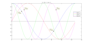 Figure 6.3 Plots of [latex]e^{-j \frac{2 \pi}{N} n * k }[/latex] for N =128, n = 0 to 127, and k = 1, 2.
Note that the points tagged in the graph represent the real part of the basis function for four points that are at
k =1 at n = 20, k = 1 at n = (20+64) = 84, k = 2 at n = 25 and k = 2 at n = (25+64) = 89
In the k = 1 case we can see that the real, and also the imaginary parts, are the negative of each other, while in the case of k = 2, the real and imaginary parts are same at each point. In order to exploit these symmetries we will divide the frequencies into even and odd values k = 2 r and k = 2 r + 1, where r goes from 0 to N/2-1.
We first work through k = 2r or even.
[latex]X(2r) = \sum_{n=0}^{\frac{N}{2}-1} ( x(n) + (-1)^{2r} * x( n + \frac{N}{2} ) ) * e^{-j \frac{2 \pi}{N} 2 * r * n} [/latex]
and since [latex](-1)^{2r} = ((-1)^2)^r = 1[/latex] we have
[latex]X(2r) = \sum_{n=0}^{\frac{N}{2}-1} ( x(n) + x( n + \frac{N}{2} ) ) * e^{-j \frac{2 \pi}{\frac{N}{2}} r * n} [/latex]
Which is a half length ([latex]\frac{N}{2}[/latex]) DFT or [latex]( x(n) + x( n + \frac{N}{2} ) )[/latex]
In a similar fashion when k is odd, we have
[latex]X(2r) = \sum_{n=0}^{\frac{N}{2}-1} ( x(n) + (-1)^{2r+1} * x( n + \frac{N}{2} ) ) * e^{-j \frac{2 \pi}{N} (2r+1) * n} [/latex]
Noting that [latex](-1)^{2r+1} = -1[/latex] we have
[latex]X(2r) = ( \sum_{n=0}^{\frac{N}{2}-1} ( x(n) - x( n + \frac{N}{2} ) ) * e^{-j \frac{2 \pi}{\frac{N}{2}} r * n} ) e^{-j \frac{2 \pi}{\frac{N}{2}} n }[/latex]
Similar to before, the summation is a half-length DFT of $latex ( x(n) – x( n + \frac{N}{2} ) )$ , however the result of each summation is multiplied by [latex]e^{-j \frac{2 \pi}{\frac{N}{2}} n }[/latex].
One of the restrictions that was placed on the length of the transform when this process started was that it be a power of 2 or N = 2p. This was done so that we could take the half length transforms and divide them in half again. this would then result in four quarter-length transforms. In order to visualize all the pieces of this computation a common layout of this is a signal flow diagram. A small eight point signal flow diagram of the FFT is included here.
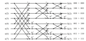
Figure 6.4 Signal Flow Diagram of an Eight Point Fast Fourier Transform.
In the signal flow diagram, a W is used instead of [latex]e^{-j \frac{2 \pi}{N}}[/latex] since that would require more space or would be too small to read.
Also, where the lines cross to do a sum and difference, these steps are commonly called butterflys. This probably comes from the appearance being similar to wings. Note when working with FFT’s a common point is the computation of these butterflys. Another feature of these butterflys is that the sum and difference can be stored back into the elements that the data was taken from. This means that the processing can be done “in place” or in the array the data was originally stored in. This greatly reduces memory requirements and the data movement operations for the computations.
Section C.1a Computational cost
The signal flow diagram in Figure 6.4, shows that the first half of x(n) is added to x(n + N/2) (x(0) + x(4), x(1) + x(5) … ) and it is done. Then the difference of the same set of points is computed and multiplied by [latex]e^{-j \frac{2 \pi}{N} n}[/latex] [ (x(0) – x(4)) * [latex]e^{-j \frac{2 \pi}{N} 0}[/latex], (x(1) – x(5)) * [latex]e^{-j \frac{2 \pi}{N} 1}[/latex] … ). Thus to complete this level requires N/2 multiplies. As we are repeatedly dividing the length by 2 and the length is 2p, we will have p (log2 N) levels and the total number of multiplies would be N/2 * log2(N), while the original sum would require N2 multiplies. In the example above (N=8) the FFT requires 4*3 (12) multiplies and the original sum would 8*8 (64) which is a factor of over 5 times as much. This factor gets even larger as N increases, for example if N = 256 the FFT would need 128*8 = 1024 and direct computation would be 2562 = 65536 which is a factor of 64.
It should be noted that the indexes of the transforms are out of order. This is due to the constant separation of the sequence into even and odd indices. Because of the nature of this process, the numbering has a binary nature. The outputs of the FFT have been numbered based on the frequency they represent. Then the frequency index number is written out in binary. On the far right hand side of Figure 6.4 it can be seen that if we reverse the bits in the binary number we will have a natural sequence from 0 to 8. This ordering is commonly called bit-reversed and can often be a computationally costly step. It is a commonly noted in numerical analysis that the computer spends from 80 to 90 percent of its time doing data moves, branch tests, … instead of the actual numerical computations. The FFT is no exception.
As a final note, the same process can be applied in the computation of the inverse DFT, with the two points. First the basis function is now [latex]e^{j \frac{2 \pi}{N}}[/latex] , noting the sign change on “j”. The same steps occur except we have “+j” instead of “-j”. Secondly, the divide by N ( the number of points in the sequence) is, by convention only, applied at the inverse DFT.
Section C.2 Transforming Signals of Other Lengths
The previous algorithm was done assuming the length of the DFT was a power of two. This length restriction can, in some cases, be too restrictive, and to address this need we can alter the previous process by decomposing the length into its prime factors. Note any integer can be written as a set of prime number raised to a power. For example a length of 24, which can be written as 23 * 31. Then the first step might be to divide the sequence into thirds, with 3*r, 3*r+1 and 3*r+2, in which case a similar simplification will result in three transforms of 1/3 the length of the original. It is true however that the power of two lengths are the most efficient, both computationally and post-weave (bit-reversed order).
Often it is helpful to see an algorithm implemented. Appendix C contains an implementation of the FFT for a power of 2, and will bring these steps together, showing how they work in the C programming language.
Section D. DFT Applications
As with the FT for continuous signals, the DFT can be used to filter and analyze discrete signals, however many of the properties of the DFT need to be kept in mind when applying the DFT. The first property we will address the is the implied periodicity of the DFT. Another property that will have to be considered is the symmetry of DFT, which will heavily affect the filters applied. Finally we will look at how the DFT can be used to measure the underlying frequency in a signal.
Section D.1 DFT Filtering and Implied Periodicity
As with the continuous FT, a filter can be characterized by the relationship
[latex]Y( \omega ) = X( \omega ) H( \omega )[/latex]
where [latex]Y( \omega )[/latex] is the FT of the output, [latex]X( \omega )[/latex] is the FT of the input, and [latex]H( \omega )[/latex] is the frequency response of the filter.
Similarly the discrete version is
[latex]Y( k ) = X ( k ) H(k)[/latex]
where [latex]Y( k )[/latex] is the DFT of the output, [latex]X( k )[/latex] is the DFT of the input, and [latex]H( k )[/latex] is the transfer function of the filter evaluated at k.
As was stated previously, when using the DFT to filter a signal, the periodicity and symmetry of the DFT must be kept in mind. The primary point here will be that we will want Y( k ) to have the proper symmetry so we have a real-valued and consistent result. Thus X( k ) and H( k ) need to have the prerequisite symmetry as well. This will occur naturally for the transformed input since we will be computing the DFT of an input signal and the DFT equations will create the proper transform. However the filter response will need to have this symmetry, such that the output transform ( X(k) * H(k) ) will be properly real-valued.
The first example of using the DFT for filtering will use a simple signal that has a slope at the start and then levels out. This constructed signal will then be filtered with a 128 point moving average filter, via the DFT.
% start with a clean slate
clear
close all
% time indexes
t = (0:2047)*100e-6;
% constructed signal
x = [(0:1023) 1023*ones( 1, 1024)]’;
% DFT filtering with 128 point moving average.
X = fft( x );
Y = fft( ones(128,1)/128, 2048 );
x1 = ifft( X.*Y );
% plot results.
plot( t, x, ‘b’, t, x1, ‘r’)
title( ‘Constructed signal and DFT filtered’ );
xlabel( ‘time (10 kHz sampling)’ );
ylabel( ‘Amplitude’);
legend( ‘Input’, ‘Filtered’ );
xlim( [0 0.2047] )
grid
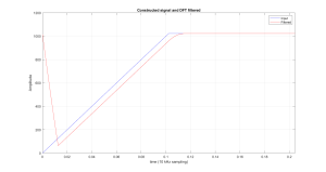
Figure 6.5 Filtered Signal, Emphasizing The Periodic Assumption in The DFT.
The plot in Figure 6.5, demonstrates how the implied assumption of periodicity can affect the results of DFT filtering. At the start of the filtered output (time 0), we see the output falling from its peak down to almost zero. To explain how this happens consider Figure 6.6, where the input to this filtering process is shown as it appears to the algorithm, with its periodic extension.
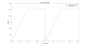
Figure 6.6 Periodic Extension of Constructed Signal
Also included in Figure 6.6, is the impulse response for the moving-average filter. The impulse response is actually set at just past t = 0, so as to emphasis how the portion for t<0, wraps into the next part of the signal. This will be shown more graphically in the following video.
One approach to fixing this periodicity problem is to append zeros onto the signal prior to the DFT. The adding of zeros at the end of a signal prior to the DFT is commonly called zero padding, and can be done in MATLAB by simply requesting a transform that is longer than the input signal. The following script will filter the same signal as was done previously, except the transforms are twice as long via zero-padding.
%% DFT filtering but padding input
Xp = fft( x, 4096 );
Yp = fft( ones(128,1)/128, 4096 );
x1p = ifft( Xp.*Yp );
% Plot results.
figure
plot( t, x, ‘b’, (0:4095)*100e-6, x1p, ‘r’ )
title( ‘Constructed signal and DFT filtered’ );
xlabel( ‘time (10 kHz sampling)’ );
ylabel( ‘Amplitude’);
legend( ‘Input’, ‘Filtered’ );
xlim( [0 0.4095] )
grid
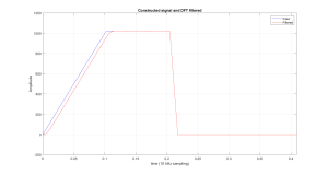
Figure 6.6 Filtered Signal With Zero Padding.
Section D.2 DFT Filtering Using H(k)
We can also produce a filter in the frequency domain by computing the frequency response of our filter at each frequency index. The most important part of the H(k) will be the Hermitian symmetry or complex-conjugate symmetry. This symmetry requires meticulous programming in the calculation of H(k). However even with the most exacting coding, small numerical errors can cause asymmetries that will cause the output to have small but meaningful imaginary parts. In the following example, another approach will be shown, along with how small of an error in the symmetry of H(k) can cause trouble with the filter’s output.
We start by generating a
% Example of applying a filter to a signal in the DFT domain.
% First, we generate a test signal, which is a frequency modulated signal.
% Compute its transform
FM = fft( fm );
% and construct a normalized frequency array ( 0 to 1 matches 0 to fs )
f = [0:length(FM)-1]/length(FM);
% We then apply bandpass and fm detector filters to the transform.
BP_FM = FM .* BandPass_dft( length( FM ) );
DET_FM = FM .* fm_det( length( FM ) );
% Display the Tranform and the filtered Transforms.
figure(1)
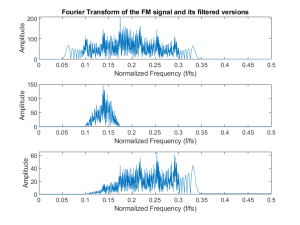
subplot( 311 ), plot( f(1:end/2), abs( FM(1:end/2)));
ylabel( ‘Amplitude’ );
xlabel( ‘Normalized Frequency (f/fs)’ );
title(‘Fourier Transform of the FM signal and its filtered versions’);
subplot( 312 ), plot( f(1:end/2), abs( BP_FM(1:end/2)));
ylabel( ‘Amplitude’ );
xlabel( ‘Normalized Frequency (f/fs)’ );
subplot( 313 ), plot( f(1:end/2), abs( DET_FM(1:end/2)));
ylabel( ‘Amplitude’ );
xlabel( ‘Normalized Frequency (f/fs)’ );
%Compute the Inverse to see the output of this type of signal.
bp_fm = ifft( BP_FM );
% Then test the imaginary part of the output to verify symmetry.
max( imag( bp_fm ) )
% ans = 0
% this is exceptionally lucky to get 0,
% Usually it need to be compared with the numerical accuracy of the system,
% given by eps
% eps = 2.2204e-016
% Repeat for FM detector.
det_fm = ifft( DET_FM );
max( imag( det_fm ) )
% ans = 0
% this is again exceptionally lucky to get 0,
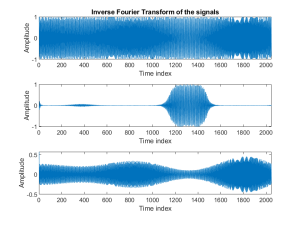
%% Display output signals.
figure(2)
subplot( 311 ), plot( fm );
ylabel( ‘Amplitude’ );
xlabel( ‘Time index’ );
xlim( [0 2047] );
title(‘Inverse Fourier Transform of the signals’);
subplot( 312 ), plot( real( bp_fm ) );
ylabel( ‘Amplitude’ );
xlabel( ‘Time index’ );
xlim( [0 2047] );
subplot( 313 ), plot( real( det_fm ) );
ylabel( ‘Amplitude’ );
xlabel( ‘Time index’ );
xlim( [0 2047] );
%% Now show what happens when you are off by one.
bp_fm_wrong = ifft( FM .* BandPass_dft_wrong( length( FM ) ) );
max( imag( bp_fm_wrong ) )
% ans = 0.0075
% Note this is 13 orders of magnitude larger that eps……
The following are the three functions called by the previous script.
The resulting plots are shown here. In the first plot we can see that the signal contains a wide range of frequencies. Once we filter it we see that the