Appendix A. Laplace and z Transform Properties.

The Laplace transform of the time function x(t) is defined as

[latex]X(s) = \int_{0}^{\infty} x(t) e^{st} dt[/latex]                                      (A.1)

Now all the intricacies and properties of this transform are derived and catalogued in a number of texts.  However in this description, we will look at the most basic and important properties.

In electrical engineering, we will be solving for voltages and currents in a circuit.  These properties are commonly described by a differential equation.  Thus one of the most useful properties is the Laplace transform of the derivative of a function.

Laplace Transform of a derivative and a System.

Let X(s) be the Laplace transform of the function of x(t) then

L{ [latex]\frac{dx(t)}{dt} [/latex] } = s X(s) + x(0)                                              (A.2)

An example of how this property of the Laplace transform can be used is the solution of the following circuit.

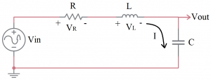
Figure A.1 Circuit Used to Demonstrate The Application of The Laplace Transform.

Applying the Kirchhoff Voltage Law (KVL) around the circuit, we have

[latex]- V_{in} + V_R + V_L + V_{out}  = 0[/latex]                      (A.3)

Recalling from physics, the voltage on the resistor (R) and inductor (L) are [latex]I*R[/latex] and [latex]L \frac{d I}{dt}[/latex] respectively.  Applying these properties to equation A.3 and solving for [latex]V_{in}[/latex] we have

[latex]V_{in} =L \frac{d I}{d t} + I * R + V_{out} [/latex]                      (A.4)

Note that in this circuit,  [latex]I = C* \frac{V_{out}}{dt}[/latex] and  thus [latex]\frac{d I}{dt} = C* \frac{{V_{out}}^2}{d^2 t}[/latex] resulting in

[latex]V_{in} = L C \frac{{V_{out}}^2}{d^2 t} +  R C \frac{V_{out}}{dt} + V_{out}[/latex]                      (A.5)

Equation A.5 is a classic Linear Time-Independent Differential Equation (LTIDE) and applying the Laplace transform to each side of the equation we have

[latex]V_{in}(s) = L C s^2 V_{out}(s) + R C s V_{out}(s) + V_{out}(s)   [/latex]                                            (A.6)

Then factoring out the [latex]V_{out}(s)[/latex] on the right hand side, we have

[latex]V_{in}(s) = ( L C s^2 + R C s + 1 ) V_{out}(s)[/latex]                                             (A.7)

This is commonly written as [latex]V_{out}(s)[/latex] as a function of [latex]V_{in}(s)[/latex], resulting in

[latex]V_{out}(s) = \frac{1}{( L C s^2 + R C s + 1 ) } V_{in}(s) [/latex]                                           (A.8)

Which is is commonly written as

[latex]V_{out}(s) = H(s) V_{in}(s)   [/latex]                                      (A.9)

And  [latex]H(s)[/latex] is referred to as the transfer function, transferring  [latex]V_{in}[/latex] to [latex]V_{out}[/latex].

Laplace Transform and Frequency Responses

[latex]H(s)|_{s=j \omega}[/latex]