Appendix B: Analog Filter Design
Analog Filters
Dwight Day
Analog Filter Design
In this chapter we will be developing filters that employ feedback of the output. These filters are commonly called Infinite Impulse Response filters (IIR), since the impulse response will extend out to infinity. To start we will review the design of Analog filters. Later a translation will be introduced to go from an analog design to a discrete design.
Section A) Filter Specifications.
Before trying to design a filter the first step needs to be to define or describe the type of filter that is to be designed. Defining the response that you will want in your filter will be a function of how it is to be used and is beyond the scope of this discussion. It is sufficient to currently break the types of filter into the three basic types of Low-Pass (LP), High-Pass (HP) and Band-Pass (BP) filters. We will find that each type can be sufficiently described by just a few values.
Part 1) Low-Pass Filter
A sketch of the frequency response of a LP filter is shown in Figure I-1. In this sketch we see that the important values are 1) the upper frequency of the pass band (wp in Figure 5.1.), the lower frequency of the stop-band (ws), and the attenuation’s for each band.
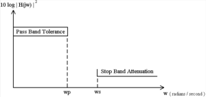
Figure 5.1 Sketch of The Frequency Response of A Low-Pass Filter.
Part 2) High-Pass Filter
A sketch of the frequency response of a HP filter is shown in Figure 5.2. This type of filter can be characterized in a fashion similar to that of the LP filter, requiring the 1) the upper frequency of the stop band (ws), the lower frequency of the pass-band (ws), and the attenuation’s for each band.
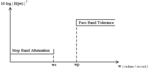
Figure 5.2 Sketch of The Frequency Response of A High-Pass Filter.
Part 3) Band-Pass Filter
A band-pass filter is more complex that the LP and HP, but can still be represented by a small set of values. Figure 5.3 contains a sketch of the BP frequency response. With the whole specification being set by the end of the lower stop band (wsl), the lower end of the pass band (wpl), the upper end of the pass band (wpu) and the end of the upper stop band (wsu).
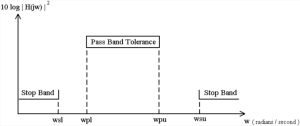
Figure 5.3 Sketch of The Frequency Response of A Band-Pass Filter.
Section B) Translation to a Normalized Low-Pass Filter
Once the design has been described in one of the previously mentioned forms, each design will be translated to a Normalized Low-Pass (NLP) filter specification. This is done to allow us to identify the proper NLP design that will match our filter once it is translated.
Part 1) Low-Pass Filter to Normalized Low-Pass
The translation that converts a NLP filter, with Laplace variable [latex]\hat s[/latex], to a general LP filter with cutoff or pass-band cutoff frequency of [latex]wp[/latex], is given in formula (5.1)
[latex]\hat s = \frac{s}{wp}[/latex] (5.1)
This translation will be used to change the H( [latex]\hat s[/latex] ) of the NLP into a LP H(s). However when we translate the NLP, the frequency response is warped to give us our desired response. The frequency warping can be characterized by the following two example points. For [latex]s = \pm j wp [/latex], which translate to [latex]\hat s = \pm j \frac{wp}{wp} = \pm j[/latex]. Also, [latex]s = \pm j ws[/latex], [latex]\hat s = j \frac{ws}{wp}[/latex]. This translation is shown graphically in Figure 5.4.
![]()
Figure 5.4 Low-Pass To Normalized Low-Pass Translation.
Part 2) High-Pass Filter to Normalized Low-Pass
The translation for a HP to NLP is a little more complex, but not that bad. The translation given it equation 2, will take the NLP H(s) and translate it to a HP filter with cutoff of wp.
[latex]\hat s = \frac{wp}{s}[/latex] (5.2)
Using this translation, [latex]s = +j wp , \hat s \frac{wp}{j wp} = \mp j[/latex] . Note: the sign of s will flip, in other words for s = +j wp, s’ = – j. Also, s = + j ws, s’ = -/+ j wp / ws. This translation is shown graphically in Figure 5.5
![]()
Figure 5.5 Sketch of HP to NLP Translation.
Part 3) Band-Pass Filter to Normalized Low-Pass
The third translation is the most complex; however, we are trying to translate from a band pass filter to a NLP, which is no small feat. The translation can be achieved via equation 5.3.
[latex]\hat s = \frac{(s^2 + wc^2)}{s wb}[/latex] (5.3)
where [latex]wc = \sqrt{ wpu * wpl }[/latex] and [latex]wb = ( wpu - wpl )[/latex]
Again, [latex]\hat s[/latex] is the Laplace variable for the NLP and s the Laplace variable for the BP filter. Let’s consider the four critical frequencies of wpl, wpu, wsl and wsu.
For s = + j wpu,
[latex]\hat s = \frac{(-wpu^2 + wpu * wpl )}{ ( + j wpu ( wpu - wpl ) )} [/latex]
[latex]\hat s = \frac{- wpu ( wpu - wpl ) }{ j wpu ( wpu - wpl ) } [/latex]
[latex]\hat s = \frac{-1 }{ + j } = + j[/latex]
For s = + j wpl,
[latex]\hat s = \frac{-wpl^2 + wpu * wpl }{+ j wpl ( wpu - wpl ) }[/latex]
[latex]\hat s = \frac{- wpl ( wpu - wpl )}{+ j wpl ( wpu - wpl )} [/latex]
[latex]\hat s = \frac{1 }{ + j } = \mp j [/latex]
Note that the sign is reversed in the last equation, in other words for -j wpl, we get +j and for
+j wpl, the result is -j.
For s = + j wsu,
[latex]\hat s = \frac{-wsu^2 + wpu * wpl }{ + j wsu ( wpu - wpl )} [/latex]
[latex]\hat s = \frac{\mp j ( wpl * wpu - wsu2 )}{ wsu ( wpu - wpl ) } [/latex]
Since wsu > wpu > wpl, the ratio in the previous equation will be negative, which mean no sign reversal will occur.
The last case will be s = + j wsl,
[latex]\hat s = \frac{ -wsl^2 + wpu * wpl}{ + j wsl ( wpu - wpl ) } [/latex]
[latex]\hat s = \frac{\mp j ( wpl * wpu - wsl2 ) }{ wsl ( wpu - wpl ) }[/latex]
However in this case wsl < wpl < wpu, which makes the ratio in the previous equation positive, which means that there will be a sign reversal.
These four cases are then shown graphically in Figure 5.6.
![]()
Figure 5.6. Sketch of BP to NLP Translation.
Where A is equal to the minimum of [latex]\frac{ wpl * wpu - wsl2}{ wsl ( wpu - wpl ) }[/latex] and [latex]\frac{wpl * wpu - wsu2 }{ wsu ( wpu - wpl )}[/latex], and B is the maximum of these two terms.
In review, it should be pointed out that the translations given by equations 1, 2, and 3 will be used to translate an H(s) for a NLP filter into either an LP, HP or BP filter. So in order to pick the correct NLP filter such that once we translate it into one of the three forms, we obtain the proper filter, we will first translate the specification as was described here.
Then using [latex]e^{-j \frac{2}{3} \pi} = e^{j \frac{4}{3} \pi }[/latex] we have
limit = 5;
% Set up s plane as real and imaginary parts of s
[x,y] = meshgrid( -2.25:0.05:0, -2.25:0.05:2.25 );
s = x + 1i*y;
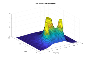
% Compute H(s) for third-order Butterworth
H = ( 1 ./ ( s + 1 ) ) .* ( 1 ./ ( s.*s + s + 1 ) );
surf( y,x,min(abs(H3),limit));
view( [ 155 45]);
title (‘H(s) of Third Order Butterworth’);
xlabel( ‘Imaginary’ );
ylabel( ‘Real’);
Another class of NLP filters are based on the Chebyshev polynomials. The Chebyshev polynomials are defined as follows,
[latex]C_n(x) = cos( n arccos( x ) )[/latex] for |x| < 1
and [latex]cosh( n arccosh( x ) )[/latex] for |x| > 1
These really are polynomials and can be generated by the recursion
[latex]C_{n+1}(x) = 2 x C_n(x) - C_{n-1}(x)[/latex]
From the definition,
[latex]C_0(x) = 1[/latex]
[latex]C_1(x) = x[/latex]
[latex]C_2(x) = 2 x C_1(x) - C_0(x) = 2 x^2 - 1[/latex]
[latex]C_3(x) = 4 x^3 - 3 x[/latex]
We will then define the frequency response of the Chebyshev filter as being
[latex]| H_{n, \epsilon}(w)|^2 = \frac{1}{( 1 + \epsilon^2 C_n^2(w) )[/latex]
where [latex]\epsilon[/latex]e is a scalar with 0 < e < 1
and [latex]C_n(w)[/latex] is the nth order Chebyshev polynomial.
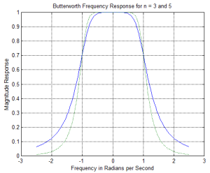
Sketches of [latex]| H_{n, \epsilon}(w)|^2[/latex] for n = 4 and 5, are included in Figure 5.10. From the plot we can see that at the cutoff frequency the filter response is not 0.707 as it was with the Butterworth, but rather a function of e. Also the response varies between 1 and [latex]\frac{1}{1+ \epsilon^2}[/latex] in the pass band (0<w<1), which gives rise to these filters other name, Equi-Ripple filters. One final point about the frequency response, if the order of the filter is even, it will have a response of 1/(1+e2) at w = 0, while if it is odd, it will have a response of 1. Also, the number of bumps is equal to the order.
The question is, how do we set e and n to match our NLP. We begin by calculating the
 Figure 5.10 Frequency Response of Chebyshev NLP Filters.
The ripple in the pass-band of the Chebyshev filter is a function of only e. The larger e, the larger the ripple and the quicker the fall off in the stop band. The Pass-Band Tolerance (PBT) will therefore set the value of e, and is a trade off situation. We will start expressing the PBT in dB, which is 20 log of the ratio of the highest gain ( 1 ) and the lowest ( [latex]\frac{1}{\sqrt{1 + \epsilon^2} }[/latex] )
[latex]PBT = 20 * log10 ( \frac{1}{ \frac{1}{ \sqrt{ 1 + \epsilon^2 } } } ) [/latex]
[latex]PBT = 20 log10 ( sqrt( 1 + \epsilon^2 ) )[/latex]
[latex]PBT = 10 log10 ( 1 + \epsilon^2 )[/latex]
[latex]\epsilon = sqrt( 10PBT/10 - 1 ) [/latex] (5.7)
Equation 5.7 is our first design equation, used to compute [latex]\epsilon[/latex] for the Chebyshev filter.
Next we will determine the order of filter needed. This equation will be derived based on the desired response at the stop frequency.
[latex]SBA = 20* log10 ( \frac{1}{\sqrt{1 + \epsilon^2 C_n^2(ws)}} ) [/latex]
[latex]SBA = -10* log10 ( 1 + \epsilon^2 C_n^2(ws) ) [/latex]
[latex]\frac{SBA}{-10} = log10 ( 1 + \epsilon^2 C_n^2(ws) ) [/latex]
[latex]C_n^2(ws) = \frac{( 10*\frac{SBA}{-10} - 1 )}{ \epsilon^2 } [/latex]
Applying the definition of Cn ,
[latex]cosh( n * arccosh( ws ) ) = \sqrt{ \frac{ ( \frac{10*SBA}{-10} - 1 )}{\epsilon} } [/latex]
Solving for n yields
[latex]n = arccosh( \sqrt( \frac{10*\frac{SBA}{-10} - 1 ) }{e} ) / arccosh( ws ) [/latex] (5.8)
Equation is the second design equation for the Chebyshev filter.
Now the reason we have defined the Chebyshev filter response as we did was because it can be shown that the polynomial [latex]( 1 + \epsilon^2 C_n^2(ws) )[/latex]will factor to have zeros at
[latex]s_k = a cos( \pi \frac{( 2 k + n - 1 )}{( 2 n ) }) + j b sin( \pi \frac{( 2 k + n - 1 )}{ ( 2 n ) }) [/latex]
where
[latex]a = 0.5 * ( (\sqrt{ 1 + \frac{1}{\epsilon^2} } + \frac{1}{e} )^{\frac{1}{n}} )- ( \sqrt{ 1 + \frac{1}{\epsilon^2} } + \frac{1}{e} )^{\frac{-1}{n}} )[/latex]
[latex]b = 0.5 * ( ( \sqrt{ 1 + \frac{1}{\epsilon^2} } + \frac{1}{e} )^{\frac{1}{n}} ) + ( \sqrt{ 1 + \frac{1}{\epsilon^2} } + \frac{1}{e} )^{\frac{-1}{n}} )[/latex]
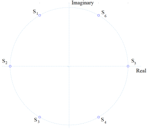
These equations are kind of tedious. Perhaps a simpler way to view them is as poles which lie on an ellipse with major and minor axis of width [latex]cosh( \frac{1}{n} arccosh(\frac{1}{e} ) )[/latex] and [latex]sinh( \frac{1}{n} arcsinh(\frac{1}{e} ) )[/latex], respectively. Figure 5.11 shows a sketch of s-plane and the general shape of the ellipse on which the poles lie.
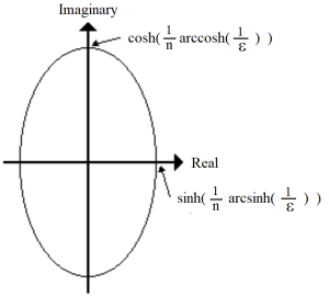
Figure 5.11 Plot of s-Plane with Chebyshev Filter Ellipse.
These poles correspond to the scaling of the real and imaginary parts of the Butterworth poles by the factors a and b, respectively. Note at 1 radian/sec, H(jw) is not equal to 0.707 or -3 dB, like the Butterworth, but rather is the ripple value.
Example: Assume a NLP filter with the following parameters is needed (PBT = 1 dB, SBA = -40dB, and ws = 10). Then
[latex]\epsilon = \sqrt{( \frac{10^1}{10} - 1 ) } = 0.5088 [/latex]
[latex]n = \frac{arccosh( \frac{( 10^{\frac{-40}{-10}} - 1 )}{\epsilon^2} ) }{arccosh( 10 )} = 1.99 [/latex]
[latex]n = 2[/latex]
The poles of this filter would now be found as follows,
a = 0.77622 and b = 1.2659
[latex]s1 = 0.77622 cos( \frac{3}{4} \pi ) + j 1.2659 sin( \frac{3}{4} \pi )[/latex]
[latex]s1 = -0.54887 + j 0.89513[/latex]
[latex]s2 = s1* = -0.54887 - j 0.89513 [/latex]
[latex]H(s) = \frac{A}{( (s-s1) (s-s2) ) } = \frac{A}{( s^2 + 1.0977 s + 1.1025 ) [/latex]
Since n is even, we know that
[latex]H(0) = \frac{A }{1.1025} = \frac{1}{\sqrt{ 1 + \epsilon^2}} [/latex]
[latex]A = \frac{1.1025}{ \sqrt{ 1 + \epsilon^2 } = 0.9826 [/latex]
[latex]H(s) = \frac{0.9826}{s^2 + 1.0977 s + 1.1025 } [/latex]
Once again we will view H(s) as a surface in the s-plane. The following is a MATLAB surface plot and script that shows H(s). Note the imaginary axis is once again the frequency response. And since the poles are pulled in closer to the imaginary axis (elliptical nature), there FR ripples more than in the case of the Butterworth.
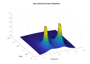
Figure 5.12 Surface plot of H(s) for Second-Order 1-dB Ripple Chebyshev NLP Filter.
================================================================
limit = 5;
% Set up z plane as real and imaginary parts of z
[x,y] = meshgrid( -2.25:0.05:0, -2.25:0.05:2.25 );
s = x + 1i*y;
H = 0.9826 ./ ( s.*s + 1.0977 * s + 1.1025 );
surf( y,x,min(abs(H),limit));
view( [ 155 45]);
title (‘H(s) of Second Order Chebyshev’);
xlabel( ‘Imaginary’ );
ylabel( ‘Real’);
================================================================
