4 Finite Impulse Response (FIR) Filter Design
Least Squares and Parks-McClellen Design
In Chapter 3 we developed the z-transform and showed that it could be used to compute the Frequency Response (FR) of a Difference Equation (DE). In this chapter we will work this somewhat in reverse, in that we will work to create a DE that implements the given FR. The first form of DE we will be working with is the feed-forward DE or the Finite Impulse Response (FIR) filter.
Section A.1) Basics of Feed-Forward Systems
The feed-forward DE can be thought of as a weighted average of the current and delayed copies of the incoming data. This process is shown graphically in Figure 4.1,
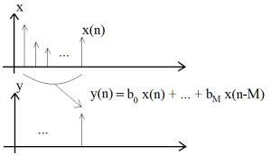
Figure 4.1 Feed-Forward As a Weighted Sum.
or as a signal-flow graph
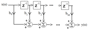
Figure 4.2 Feed-Forward Signal-Flow Graph
In equational form this works out to be
[latex]y(n) = b_0 * x(n) + b_1 * x(n-1) + ... + b_M * x(n-M)[/latex] (4.1)
or
[latex]y(n) = \sum_{k=0}^{M}{b_k * x(n-k)} [/latex] (4.2)
Taking the z-transform of equation 4.2, we will have
[latex]Y(z) = \sum_{k=0}^{M}{b_k * z^{-k} } X(z)[/latex] (4.3)
Writing this in the more classical form as
[latex]Y(z) = H(z) X(z)[/latex] (4.4)
where [latex]H(z) = \sum_{k=0}^{M}{b_k * z^{-k} }[/latex]
Of course the real objective will be have a filter with a given FR. We have established that the FR of a z-transform can be found by evaluating the H(z) at [latex]e^{j \omega}[/latex] or [latex]e^{j 2 \pi \frac{f}{f_s}}[/latex] where [latex]\omega[/latex] goes from [latex]-\pi[/latex] to [latex]\pi[/latex], which will match up to [latex]f[/latex] going from [latex]-\frac{f_s}{2}[/latex] to [latex]\frac{f_s}{2}[/latex].
[latex]H(e^{j 2 \pi \frac{f}{f_s} } = \sum_{k=0}^{M}{b_k e^{-j 2 \pi k \frac{f}{f_s}}}[/latex] (4.5)
In the next section we will define some basic structure that is needed in order to properly set the [latex]b_k[/latex]‘s to build a desired FR.
Section A.2) Types of Feed-Forward Systems
Of course the real objective will be have a filter with a given FR. We have established that the FR of a z-transform can be found by evaluating the H(z) at [latex]e^{j \omega}[/latex] or [latex]e^{j 2 \pi \frac{f}{f_s}}[/latex] where [latex]\omega[/latex] goes from [latex]-\pi[/latex] to [latex]\pi[/latex], which will match up to [latex]f[/latex] going from [latex]-\frac{f_s}{2}[/latex] to [latex]\frac{f_s}{2}[/latex].
As an example, consider a five-point weighting of [latex]b_0, b_1, b_2, b_3,[/latex] and [latex]b_4[/latex]. The FR of which is
[latex]H(e^{j 2 \pi \frac{f}{f_s}}) = b_0 e^{-j 0 } + b_1 e^{-j 2 \pi f} + b_2 e^{-j 4 \pi f} + b_3 e^{-j 6 \pi f} +b_4 e^{-j 8 \pi f} [/latex]
It should be noted that [latex]f_s[/latex] has been set to 1, to simplify the equations. So now in order to make this FR meaningful, we will factor out [latex]e^{- j 4 \pi f}[/latex]
[latex]H(e^{j 2 \pi f}) = e^{-j 4 \pi f} ( b_0 e^{j 4 \pi f } + b_1 e^{j 2 \pi f} + b_2 e^{-j 0} + b_3 e^{-j 2 \pi f} +b_4 e^{-j 4 \pi f} [/latex]
and reorder these terms, to yield
[latex]H(e^{j 2 \pi \frac{f}{f_s}}) = e^{-j 4 \pi f} ( b_0 e^{j 4 \pi f } +b_4 e^{-j 4 \pi f} + b_1 e^{j 2 \pi f} + b_3 e^{-j 2 \pi f} + b_2 e^{-j 0} ) [/latex]
From this we can see that if we have [latex]b_0 = b_4[/latex] and [latex]b_1 = b_3[/latex] we will have
[latex]H(e^{j 2 \pi \frac{f}{f_s}}) = e^{-j 4 \pi f} ( b_0 ( e^{j 4 \pi f } + e^{-j 4 \pi f} ) + b_1 ( e^{j 2 \pi f} + e^{-j 2 \pi f} ) + b_2 e^{-j 0} )[/latex]
and employing one of Euler’s identities ( [latex]2 cos( x ) = e^{j x} + e^{-j x}[/latex] ) and reordering
[latex]H(e^{j 2 \pi f}) = e^{-j 4 \pi f} ( b_2 + b_1 * 2 cos( 2 \pi f) + b_0 * 2 * cos(4 \pi f) )[/latex]
The main take away from this is the following point. If we have symmetry in our weights ([latex]b_0 = b_4[/latex]), commonly referred to as even symmetry, the FR reduces to a linear phase angle ([latex]e^{-j4 \pi f}[/latex], whose magnitude is 1 ) and a real valued magnitude ( [latex]( b_2 + b_1 * 2 cos( 2 \pi f) + b_0 * 2 * cos(4 \pi f) )[/latex], which sufficiently general enough to match a wide range of FR). This will greatly simplify the design process allowing us to match a variety of FR’s, given a sufficient number of weights.
As a kind of counter point, what if we were to have an odd symmetry of [latex]b_0 = -b_4[/latex] and [latex]b_1 = -b_3[/latex] we will have
[latex]H(e^{j 2 \pi \frac{f}{f_s}}) = e^{-j 4 \pi f} ( b_0 ( e^{j 4 \pi f } - e^{-j 4 \pi f} ) + b_1 ( e^{j 2 \pi f} - e^{-j 2 \pi f} ) + b_2 e^{-j 0} )[/latex]
and employing one of Euler’s identities ([latex]2 j*sin( x ) = e^{j x} - e^{-j x}[/latex]) and reordering
[latex]H(e^{j 2 \pi f}) = e^{-j 4 \pi f} ( b_2 + b_1 * 2 j * sin( 2 \pi f) + b_0 * 2 * j * sin(4 \pi f) )[/latex]
And to avoid the real and complex terms on the right hand side, we should set [latex]b_2 = 0[/latex] and let [latex]j = e^{j \frac{\pi}{2}}[/latex] resulting in
[latex]H(e^{j 2 \pi f}) = e^{-j 4 \pi f + \frac{\pi}{2}} ( b_1 * 2 * sin( 2 \pi f) + b_0 * 2 * sin(4 \pi f) )[/latex]
Unfortunately this not as general a solution as what the even symmetry was providing us.
Having odd symmetry ([latex]b_k = -b_{-k}[/latex]) results in a Type III Filter
Type II and Type IV filter have similar restrictions
Not meaningful at this time.
Section A.3) Feed-Forward Systems as Convolutions
It was stated previously that we can look at these systems as weighted sum of the incoming data. Another way to look at this is as a convolution of the incoming sequence with weights [latex]b_k[/latex].
Now convolution is one of those techniques that when you learn about it you probably don’t expect to ever use it or need it. Well in the case of discreet data, it proves to be an exceptionally good mental model, if nothing else. So as part of this the following video show a convolution in sequence. And will introduce the frequency response.
[latex]H(e^{j 2 \pi f}) = \frac{1}{3} e^{-j 0 } + \frac{2}{3} e^{-j 2 \pi f} + e^{-j 4 \pi f} + \frac{2}{3} e^{-j 6 \pi f} + \frac{1}{3} e^{-j 8 \pi f} [/latex]
Video Code
% Start with a clean slate
close all
clear
% Creating input and output arrays.
x = zeros(100,1);
y = x;
x(6:30) = sin( 2*pi*(0:24)/25 ); % low frequency sin wave
x(31:55) = sin( 2*pi*(0:24)/12.5 ); % mid frequency sin wave
x(56:80) = sin( 2*pi*(0:24)/6.25 ); % high frequency sin wave
% Shape of filter weights/impulse response.
w = ([0 1 2 3 2 1 0]/3)’;
k = 7; % start is offset to simplify convolution computation.
% loop.
while k < 100
y(k) = sum( w.*x(k-6:k)); % convolution (cross multiply and sum)
% plot input and filter, and output up to k
subplot( 211 ),plot( k-6:k, w, ‘r’, 0:99, x, ‘b’ );
title( ‘Input and Filter Response’ );
legend( ‘Filter Response’, ‘Input’);
subplot( 212 ),plot( y );
title( ‘Output at Each Stage’ );
% pauses
if k == 7
pause; % pause waiting to start.
else
if k < 25
pause( 1 ); % slow at first
else
pause( 0.25 ); % faster.
end
end
k = k + 1; % move to next point.
end
Here in Section A, we have tried to describe the structure of a Feed-Forward system and how
Section B.1) Derivation of the Least Squares or Fourier Series Design of an FIR filter
Which brings us to the fact that for a filter of this type, the transfer function is
[latex]H(z) = \sum_{k=0}^{-M}{b_k * z^{-k}}[/latex] (4.6)
We will now look at the FR of this transfer function.
[latex]H(e^{j \omega} T) = \sum_{k=- \infty}^{\infty}{b_k e^{j k \omega T}}[/latex] (4.7)
It should be noted that in the equation for the FR, we also changed the sum to go from [latex]- \infty[/latex] to [latex]\infty[/latex] instead of 0 to M. Although this represents data from the future, in the setting of our analysis we will be able to work this through. Perhaps we should just think of it as delaying the output.
[latex]H(e^{j \frac{\omega_o}{f_s}}) = \sum_{k=- \infty}^{\infty}{b_k e^{j k \frac{\omega_o}{f_s}}}[/latex] (4.7)
Let [latex]\omega_o = 2 \pi f_o[/latex] then we have
[latex]H(e^{j 2 \pi \frac{f_o}{f_s}}) = \sum_{k=- \infty}^{\infty}{b_k e^{j 2 \pi k \frac{f_o}{f_s}}}[/latex] (4.8)
Although it is not readily obvious, equation 4.8 can actually be looked at as a Fourier Series (FS), where the role of time and frequency have been reversed. This reversal is possible, since the FR of a discrete system is periodic (Chapter 2).
With that said we can employ the FS to solve for [latex]b_k[/latex] using the integral formula
[latex]b_k =\frac{1}{f_s} \int_{f=-\frac{fs}{2}}^{\frac{f_s}{2}}{H_d(e^{j 2 \pi f }) * e^{j k 2 \pi \frac{f}{f_s}}} df[/latex] (4.9)
where [latex]H_d(e^{j 2 \pi f })[/latex] represents our desired FR.
Example
Consider the following sketch of an idealized band-pass filter. If we were to apply equation 4.9 we have
[latex]b_k = \frac{1}{2 \pi} \int_{f=-\pi}^{\pi}{H_d(e^{j \omega}) * e^{j \omega f}} d\omega[/latex]
Before we apply this in an example, it should be noted that to insure that the [latex]b_k[/latex]‘s are real valued we will require that [latex]H_d(e^{j 2 \pi f })[/latex] have an even magnitude ([latex]| H_d(e^{j 2 \pi f }) | = | H_d(e^{-j 2 \pi f }) |[/latex]) and an odd phase ([latex]\angle H_d(e^{j 2 \pi f }) = - \angle H_d(e^{-j 2 \pi f })[/latex])
A simple example of this is shown here.
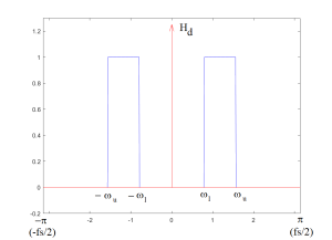
Figure 4.3 Idealized Band-Pass Filter
Since Hd is zero most of the time and 1 in the two intervals the integral becomes
[latex]b_k = \frac{1}{2 \pi} [ \int_{f=-\omega_u}^{-\omega_l}{H_d(e^{j \omega}) * e^{j \omega f}} + \int_{f=\omega_l}^{\omega_u}{H_d(e^{j \omega}) * e^{j \omega f}} ] d\omega[/latex]
The integral is relatively simple and evaluates to
[latex]b_k = \frac{1}{2 \pi} [ ( \frac{e^{j\omega k}}{j k}|_{\omega=-\omega_u}^{-\omega_l} + ( \frac{e^{j\omega k}}{j k}|_{\omega=\omega_l}^{\omega_u} ][/latex]
Complete the evaluation of the integral we have
[latex]b_k = \frac{1}{2 \pi} [ \frac{e^{-j\omega_l k}-e^{-j\omega_u k}}{j k} + ( \frac{e^{j\omega_u k}-e^{j\omega_l k}}{j k} ][/latex]
Then we reorder the equation grouping [latex]\omega_l[/latex] and [latex]\omega_u[/latex], to produce
[latex]b_k = \frac{1}{2 \pi} [ \frac{e^{-j\omega_l k}-e^{j\omega_l k}}{j k} + ( \frac{e^{j\omega_u k}-e^{-j\omega_u k}}{j k} ][/latex]
Employing one of the Euler identities ( [latex](e^{jx} - e^{-jx}) = 2 j * sin( x )[/latex] ) produces
[latex]b_k = \frac{1}{2 \pi} [ \frac{-j2 sin(\omega_l k)}{j k} + ( \frac{j2 sin(\omega_u k)}{j k} ][/latex]
Factoring out the j terms and multiplying each part of the sum by [latex]\omega_u[/latex] and [latex]\omega_l[/latex] respectively, we have
[latex]b_k = \frac{1}{2 \pi} [ \frac{\omega_u 2 sin(\omega_u k)}{ \omega_u k} + ( \frac{\omega_l 2 sin(\omega_l k)}{j \omega_l k} ][/latex]
Note the function [latex]\frac{sin(x)}{x}[/latex] is common enough that it is called [latex]sinc(x)[/latex] and cancelling out the 2’s we have
[latex]b_k = \frac{1}{\pi} [ \omega_u sinc(\omega_u k) + ( \omega_l sinc(\omega_l k) ][/latex]
A little reordering adn we have a closed form equation for our [latex]b_k[/latex] terms
[latex]b_k = \frac{\omega_u}{\pi} sinc(\omega_u k) + \frac{\omega_l}{\pi} sinc(\omega_l k) ][/latex] (4.10)
Consider this example of equation 4.10 for three filters.
First we will try a low-pass filter with [latex]\omega_l = 0[/latex] and [latex]\omega_u = \frac{\pi}{8}[/latex], which results in
[latex]h_0(k) = \frac{1}{8} sinc( \pi \frac{k}{8}) - 0 * sinc( 0 )[/latex]
Next we have a band-pass filter with [latex]\omega_l = \frac{\pi}{8}[/latex] and [latex]\omega_u = \frac{\pi}{4}[/latex], which results in
[latex]h_1(k) = \frac{1}{4} sinc( \pi \frac{k}{4}) - \frac{1}{8} * sinc( \pi \frac{k}{8} )[/latex]
We then create another band-pass filter with [latex]\omega_l = \frac{\pi}{4}[/latex] and [latex]\omega_u = \frac{\pi}{2}[/latex], producing
[latex]h_2(k) = \frac{1}{2} sinc( \pi \frac{k}{2}) - \frac{1}{4} * sinc( \pi \frac{k}{4} )[/latex]
Finally we will want to look at a high-pass filter which will have [latex]\omega_l = \frac{\pi}{2}[/latex] and [latex]\omega_u = \pi[/latex], producing
[latex]h_3(k) = sinc( \pi * k ) - \frac{1}{2} * sinc( \pi \frac{k}{2} )[/latex]
Since [latex]sinc( \pi * k ) = 1[/latex] our high-pass filter is
[latex]h_3(k) = 1 - \frac{1}{2} * sinc( \pi \frac{k}{2} )[/latex]
We will now show how these four filters work in a MATLAB script that tests them out.
Section B.2) MATLAB Design Using Our Least Squares Design of an FIR filter
In order to implement the filter, we will need to truncate the sum to only go from -N to N. It is important to keep it symmetric around 0, so
[latex]\hat H(e^{j 2 \pi \frac{f_o}{f_s}}) = \sum_{k=-N}^{N}{b_k e^{j 2 \pi k \frac{f_o}{f_s}}}[/latex]
Then to avoid have negative delays, we will shift it by N ([latex]\hat k = N + k[/latex]) so we have
[latex]\hat H(e^{j 2 \pi \frac{f_o}{f_s}}) = \sum_{\hat k=0}^{2N}{b_k e^{j 2 \pi (\hat k - N) \frac{f_o}{f_s}}}[/latex]
We can now factor to
[latex]\hat H(e^{j 2 \pi \frac{f_o}{f_s}}) = e^{- j 2 \pi N \frac{f_o}{f_s}} \sum_{\hat k=0}^{2N}{b_k e^{j 2 \pi \hat k \frac{f_o}{f_s}}}[/latex] (4.9)
From this equation we end up with the sum representing magnitude of the FR that we were designing for, and the [latex]e^{-j 2 \pi N \frac{f_o}{f_s}}[/latex] term represents a linear phase shift.
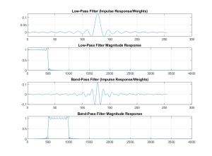
The following is a MATLAB script that will start by generating the four filters and their frequency responses.
%%%%%%%%%%%%%%%%%%%%%%%%%%%%%%%%%%%%%%%%%%%%%%%%
% Fourier Series Filter section.
%
% We start with the indices of k going from -127 to 127
% which is symmetric around 0,
n = [-127:127];
% Evaluate for the four filters.
fs0 = (1/8)*sinc( n / 8 );
fs1 = (1/8)*(2 * sinc( n / 4 ) – sinc( n / 8 ) );
fs2 = (1/4)*(2 * sinc( n / 2 ) – sinc( n / 4 ) );
fs3 = (1/2)*(2 * sinc( n ) – sinc( n / 2 ) );
% Frequency responses of the Fourier Series filters.
[FS0,w] = freqz( fs0, 1, 4096);
[FS1,w] = freqz( fs1, 1, 4096);
[FS2,w] = freqz( fs2, 1, 4096);
[FS3,w] = freqz( fs3, 1, 4096);
% Plot of the Fourier Series filters
% and the magnitude frequency response of each.
figure( 1 );
subplot( 411 ),plot( fs0 );
title(‘Low-Pass Filter (Impulse Response/Weights)’);
grid
subplot( 412 ),plot( w*4000/pi, abs( FS0 ) );
title(‘Low-Pass Filter Magnitude Response’);
grid
subplot( 413 ),plot( fs1 );
title(‘Band-Pass Filter (Impulse Response/Weights)’);
grid
subplot( 414 ),plot( w*4000/pi, abs( FS1 ) );
title(‘Band-Pass Filter Magnitude Response’);
grid
figure( 2 );
subplot( 411 ),plot( fs2 );
title(‘Band-Pass Filter (Impulse Response/Weights)’);
grid
subplot( 412 ),plot( w*4000/pi, abs( FS2 ) );
title(‘Band-Pass Filter Magnitude Response’);
grid
subplot( 413 ),plot( fs3 );
title(‘High-Pass Filter (Impulse Response/Weights)’);
grid
subplot( 414 ),plot( w*4000/pi, abs( FS3 ) );
title(‘High-Pass Filter Magnitude Response’);
grid
% Frequency responses of the Fourier Series filters.
% Testing the length.
FS0_1 = freqz( fs0(128-64:128+64), 1, 4096);
% Plot of the Fourier Series filters
% and their frequency response.
figure( 2 );
subplot( 311 ),plot( [-127:127], fs0, ‘b’,…
[-64:64], fs0(128-64:128+64), ‘r’ );
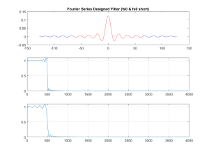
title( ‘Fourier Series Designed Filter (fs0 & fs0 short)’ );
subplot( 312 ),plot( w*4000/pi, abs( FS0 ) );
grid
subplot( 313 ),plot( w*4000/pi, abs( FS0_1 ) );
grid
Important takeaways from the previous MATLAB example.
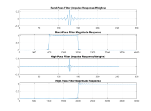
1) The first two graphs shows plots of the weights of the four designs described previously and plots the FR of each. As an extra point, the frequency responses were plotted assuming a sampling frequency of 8 KHz, thus the plots go from 0 to 4 KHz.
2) The frequency responses of the filters are not ideal, but do cutoff at the correct frequencies. And perhaps more importantly, all exceed a gain of 1 around the transitions. The rippling effect seen, again near the transition frequencies, is known as a Gibb’s phenomena.
3) The last graph is a study of the effect of the length of the filter on its FR. In this plot we use the low-pass filter and compute its FR for its full length (-127 to 127) and a shortened version (-64 to 64). The FR of these two versions of the low-pass filter show a couple important points. First, the longer the filter the sharper the transition. Second, the ripples on both filters are of similar height, but the longer filters ripples are shorter.
Section B.3) The Effect of a Window Function on a Filters FR.
The ripples on the FR of the FIR filter are the result of truncating the filter that we have generated. But to characterize this effect, we need to model it, which will allow us to control the effect more. The model that has proven quite effective is the idea of a window function. So if we consider the lowpass filter generated in the previous section,
[latex]h_0(k) = \frac{1}{8} sinc( \pi \frac{k}{8}) [/latex]
We can view the truncated form of this as
[latex]\hat h_0(k) = h_0(k) ~ w(k)[/latex]
where [latex]w(k) = \begin{bmatrix} 1 ~ for~ |k| \le \frac{N}{2} \\ 0 ~ otherwise \end{bmatrix}[/latex]
The following graph is meant as a visual description of this, showing a filter from the previous section and a square window .
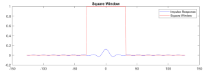
Figure 4.4 Low-Pass Impulse Response and Square Window.
Much as we did when we worked through the sampling modelling, multiplying in time causes us to convolve in the frequency domain. This convolution is described in the following formula. Starting with the form of the spectral response of the window function, which is similar to the least square filters we developed previous, or the other square functions we have worked
[latex]W( e^{j \omega } ) = \frac{1}{N} sinc( \omega )[/latex]
Then the frequency response of our filter becomes
[latex]\hat H( e^{j \omega} ) = \int_{\omega =-\infty}^{\infty}{H_d(e^{j \omega}) * W( e^{j \omega } ) } d \omega[/latex]
To demonstrate how this convolution creates the ripples seen in the frequency response of our truncated filter, the following video was created.
So is there some window that will have less of an effect on the FR of our filter. Well the most common is the Hamming window, and was constructed by noting that the ripples are all of a given width (related to the inverse of the windows length). The objective is to shift over and add these ripples together, such that the cancel each other out. The following graph shows this shifting and adding.
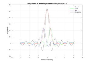
Figure 4.5 Hamming Window Construction Layout
Now the shifting is achieved by multiplying the waveform by [latex]e^{j \frac{ \pi}{N}}[/latex] where N is the length of the window. Also important is that the height of the various ripples try and cancel each other. By matching the first set of ripples it was found that the window should be
[latex]w(n) = 0.54 + 0.23 * e^{j \frac{ \pi}{N}} + 0.23 * e^{-j \frac{ \pi}{N}}[/latex]
or
[latex]w(n) = 0.54 + 0.46 * cos( \frac{ \pi}{N} )[/latex]
Which is the standard form for the Hamming window and is shown graphicallu in Figure 4.6.
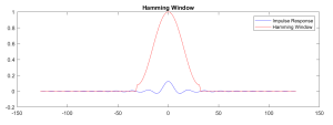
Figure 4.6. Low-Pass Filter and Hamming Window.
We will now see this effect in the form of a video showing the convolution.
Just to reiterate, the FR of two low pass filters of the same length, one has a square window (just truncated) and the other a Hamming window are plotted in the following graph. In this graph we can see that the Hamming ripples less, but transitions slower.
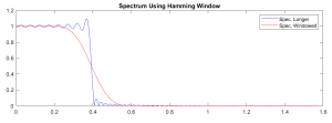
Figure 4.7 Square Window versus a Hamming Window.
Section C) Parks-McClellen (PM) Design Process.
Depending upon what linear system class you may have had, you may have been shown that the Fourier Series (FS) is actually a least-squares fit of a
[latex]\epsilon^2 = \frac{1}{2 \pi} \int_{- \pi}^{\pi}{ | H_d(e^{j \omega}) - H(e^{j \omega} ) |^2 } d \omega[/latex] ( 4.10)
The strict nature of this fit is the source of the Gibbs phenomena, noted on previously. So we will want to work towards a more general fit. Although it may not be readily obvious, we will be able to optimize the following criteria.
[latex]\delta = max_{\omega \in \{ 0:\pi \} }{ | E(\omega) | }[/latex]
where [latex]E(\omega) = W( \omega ) [ H_d(e^{j \omega}) - H(e^{j \omega}) ][/latex]
and [latex]W( \omega )[/latex] is a generic weighting function over [latex]\omega \in \{0:\pi\}[/latex] and [latex]H_d(e^{j \omega } )[/latex] is the desired response.
Since this is so general, the optimization will require a computer search in order to optimize it. We will begin by restricting the filters to have an even weighting. This restriction will result in the following
[latex]H_e(e^{j \omega}) = h_e(0) + 2 \sum_{k=1}^{\frac{M}{2}}{ h_e(k) cos( \omega k ) }[/latex] (4.11)
The even symmetry impulse has an odd number of points, including the center point at 0. As part of this process we will translate the term [latex]cos( \omega k )[/latex] into
[latex]cos( \omega k ) = T_k(cos(\omega) )[/latex]
where [latex]T_k()[/latex] is a [latex]k^{th}[/latex] order T’chebyshev polynomial. NOTE: the spelling of Russian names is not standardized and is commonly written as Chebyshev.
[latex]cos( \omega k ) = C_0 + C_1 cos(\omega) + C_2 cos(\omega)^2 + ... + C_k cos( \omega )^k[/latex] (4.12)
Merging 4.11 and 4.12 we can write this as
[latex]H_e(e^{j \omega}) = \sum_{k=0}^{\frac{M}{2}}{ a_k (cos(\omega))^k }[/latex]
Note: [latex]a_k[/latex] is a merger of [latex]h_e(k)[/latex] and [latex]C_k[/latex].
Another way to look at this is as a conformal mapping by [latex]cos(\omega)[/latex] which is a one to one mapping of [latex]\omega \in \{0:\pi\}[/latex] onto [latex]cos( \omega ) \in \{ -1:1 \}[/latex]. A graph that displays this is included here.
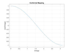
Figure 4.8 Conformal Mapping of [latex]\omega[/latex] From 0 to [latex]\pi[/latex] to 1 to -1.
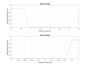
Figure 4.9 Example Frequency Response Under The cos([latex]\omega[/latex]) Mapping.
The primary reason for applying this conformal mapping is that a large number of mathematician have studied polynomials that work on the interval -1 to 1, as shown in the second plot in Figure 4.9. As was touched on above, the Chebyshev polynomials are one such set.
Now the math associated with this algorithm is rather complex, and as I have often said, not conducive to understanding. So here is my hand waving description of this process.
We set up our filter requirements, such as the cut off and stop frequencies ( [latex]\omega_c and \omega_s[/latex]). Then based on the order of filter we are wanting, we will establish a set of frequencies that are distributed through this range, as is shown in Figure 4.10. Note that [latex]\delta[/latex] is a function of the number of coefficients you have chosen for the filter. With these frequencies and such, we can fit a polynomial of [latex]cos( \omega )[/latex] through these points, sketched in Figure 4.10.
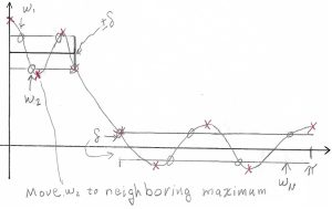
Figure 4.10 Initial Step For Parks-McClellen Design Process.
Next we fit a polynomial of [latex]cos( \omega )[/latex] versus gain, shown as a line in Figure 4.10 and going through the small circles. The local maxima and minima of that polynomial are found (mark with an x) and the frequencies are replaced with the frequencies of the maxima and minima. This changing of frequencies is known as the Remez Exchange. Thus we should have something closer to fitting the bound, as shown in (4.11).
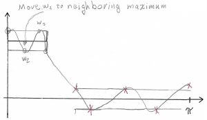
Figure 4.11 Second Iteration of Parks-McClellen Design Process.
This process will continue until the maxima and minima points all land inside the [latex]\delta[/latex] bounds. The character of the Remez exchange will converge to this point. One of main features of this type of design is the ripples in the passband and the stopband, thus in some cases these are known as equi-ripple filters. With the allowing for ripples in the bands, the PM designs tend to need fewer points than the FS designs to implement a similar filter.
We will now look at the integer math used to implement these filters.
Section D) Implementing FIR Filters – Integer Math.
Depending upon the application that the FIR filter is to be used for, the filter may need to be converted to an integer format. This is especially true if the filter is to be implemented in real-time, or with an Field Programmable Gate Array (FPGA). The process is commonly called the Qn.m format. The Q can be viewed as Quantized.
We start by recalling how we write numbers in binary and how they convert to decimal formats. In the following equation we treat a binary number ( [latex]b_7 b_6 b_5 b_4 b_3 b_2 b_1 b_0[/latex] ) as each digit represents a power of 2, thus the decimal equivalent is
[latex]b_7 b_6 b_5 b_4 b_3 b_2 b_1 b_0 => b_7 2^7 + b_6 2^6 + b_5 2^5 + b_4 2^4 + b_3 2^3 + b_2 2^2 + b_1 2^1 + b_0 2^0[/latex]
[latex]b_7 b_6 b_5 b_4 b_3 b_2 b_1 b_0 => b_7 128 + b_6 64 + b_5 32 + b_4 16 + b_3 8 + b_2 4 + b_1 2 + b_0 1 [/latex]
For example, consider the following binary number
00110101 = 0 * 128 + 0 * 64 + 1 * 32 + 1 * 16 + 0 * 8 + 1 * 4 + 0 * 2 + 1 * 1 = 32 + 16 + 4 + 1 = 53
Just to add another level of complexity to this, negative numbers are commonly represented in a 2’s complement format. In the derivation of 2’s complement representation, a negative number should have an infinite string of 1 to the left. Since we commonly work with finite length numbers, the highest bit is assumed to be the sign bit. The simplest form of this is for the sign bit to represent a negative power of 2. An example might be
[latex]b_7 b_6 b_5 b_4 b_3 b_2 b_1 b_0 => b_7 *(-2^7) + b_6 *2^6 + b_5 *2^5 + b_4 *2^4 + b_3 *2^3 + b_2 *2^2 + b_1 *2^1 + b_0 *2^0[/latex]
[latex]b_7 b_6 b_5 b_4 b_3 b_2 b_1 b_0 => b_7*-128 + b_6 *64 + b_5 *32 + b_4 *16 + b_3 *8 + b_2 *4 + b_1 *2 + b_0*1 [/latex]
Again a example is
10010101 = -128 + 16 + 4 + 1 = -107
In all of this we have assumed a binary point at the end of the number. If we assume the binary point to be just after the sign bit then the exponents of the various bits would be as shown here.
[latex]b_7 b_6 b_5 b_4 b_3 b_2 b_1 b_0 => b_7 (-2^0) + b_6 2^-1 + b_5 2^-2 + b_4 2^-3 + b_3 2^-4 + b_2 2^-5 + b_1 2^-6 + b_0 2^-7[/latex]
[latex]b_7 b_6 b_5 b_4 b_3 b_2 b_1 b_0 => b_7 (-1) + b_6 * 0.25 + b_5 * 0.125 + b_4 * 0.0625 + b_3 * 0.03125 + b_2 * 0.015625+ b_1 * 0.0078125 + b_0 * 0.00390625[/latex]
This results in numbers that can go from -1 (1000 0000 = -1) to almost 1 (0111 1111 = 1-2-7)
