The Z Transform and Its More Important Properties.

In the previous chapter we looked what happens to a signal when we reduce it to a sequence of number via an ADC.  We will now move on to the next step in our original system in which we will develop the algorithms we will be using in the processor to convert the samples coming in from the ADC into the sequence we send out to the DAC.

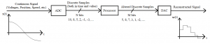
Figure 3.1 Basic Discrete Data System Layout.

Section A) Z Transform

In chapter 2, we showed how effective the Nyquist model was at characterizing data that is a sequence of samples, and that the Fourier Transform (FT) of that modelled data elucidated some very interesting properties.  We will now take that sampled data and employ the Laplace transform.  Equation 3.1 is the Laplace transform of the input x(t) times the stream of impulses that create the Nyquist sampled signal.

[latex]X_s (s) =  \int_{0} ^{\infty} (  x(t)  * \sum_{n=-\infty} ^{\infty} {\delta (t-n T)}  * e^{-s t} ) dt[/latex]                   (3.1)

We will move x(t) under the sum and then based on the sifting property of impulse functions, we replace x(t) with x(n T), since t = n T is the only place that [latex]\delta(t-n T)[/latex] is not zero.

[latex]X_s (s) =  \int_{0} ^{\infty} (  \sum_{n=-\infty} ^{\infty} {x(n T)  * \delta (t-n T) * e^{-s t} } ) dt[/latex]                   (3.2)

As was the case with the FT, we will somewhat dispense with mathematical rigor and assume the proper conditioning on the functions and interchange the summation and integral.  Do understand, this is done not to dismiss rigor, but to aid in understanding the process.

[latex]X_s (s) =  \sum_{n=-\infty} ^{\infty} (x(n T)  * \int_{0} ^{\infty} ( \delta (t-n T) * e^{-s t} ) dt)[/latex]                   (3.3)

Employing the sifting property of the [latex]\delta[/latex] function, the integral disappears and it replaced with the summation of the values at t = n T.  Resulting in

[latex]X_s (s) =  \sum_{n=0} ^{\infty} (  x(n T)  * e^{-s n T}  ) dt[/latex]                                                 (3.4)

Then we will substitute in [latex]z = e^{s T}[/latex] and remove the redundant T from x(n T) and we will  have equation 3.5

[latex]X_s (z) =  \sum_{n=0} ^{\infty} (  x(n)  * z^{-n}  )[/latex]                                                         (3.5)

This summation equation (3.5) is known as the z transform, and much like the Laplace transform it will be our tool to understand and design discrete systems.  Since the z transform is the Laplace of a sampled signal, it will provide us with similar properties and results as the Laplace, but with subtle differences.

Section A2) Examples and The Form of z Transforms

To get an understanding of what the z transform represents, let’s consider a generic signal that we will use to represent sequences.  Let

[latex]x(n) = a^n * u_s(n)[/latex]                                             (3.6)

In equation 3.6, the part [latex]u_s(n)[/latex] is known as a unit step sequence and is there to make the sequence zero for negative values of n.  The shape of this sequence is shown in Figure 3.2.

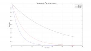
Figure 3.2 Shape of Generic Sequence for Different Values of a.

As can be seen in the previous graph, [latex]a^n[/latex] has a shape similar to the dying exponentials common with linear systems.  Thus we expect it to have a similar action.  So we will compute the z transform of this signal, which starts by inserting it into the definition of the z transform.

[latex]X_s (z) =  \sum_{n=0} ^{\infty} (  a^n  * z^{-n}  )[/latex]                                                         (3.7)

Then we rewrite the sum as

[latex]X_s (z) =  \sum_{n=0} ^{\infty} (  (a z^{-1} )^n  )[/latex]                                                         (3.8a)

or

[latex]X_s (z) =  \sum_{n=0} ^{\infty} (  (\frac{a}{z} )^n  )[/latex]                                                         (3.8b)

In eq. 3.8a and 3.8b, we are computing the sum of a geometric sequence.  Although it may not automatically come to you, the sum of a geometric sequence is known and will rederived here.

The generic form of a sum of a geometric sequence is

[latex]\sum_{n=0} ^{N-1} ( a^n  )[/latex]                                                         (3.9)

Note it is a finite sequence, but we will later have [latex]N \rightarrow \infty[/latex].

The sequence is thus

[latex]\sum_{n=0} ^{N-1} ( a^n  ) = a^0 + a^1 + ...+ a^{N-2} + a^{N-1}[/latex]                                                         (3.10)

If we multiply the sum by a, we have

[latex]a *  \sum_{n=0} ^{N-1} ( a^n  ) = a^1 + a^2 + ... + a^{N-1} + a^{N}[/latex]                                                         (3.11)

Now we take the difference 3.10 minus 3.11 and note that the second term in 3.10 is the same as the first term in 3.11.  This trend continues until the last term in 3.10, which matches the next to last term in 3.11.  Thus the difference is

[latex]\sum_{n=0}^{N-1} ( a^n  ) - a *  \sum_{n=0} ^{N-1} ( a^n  ) = a^0 - a^N[/latex]                                       (3.12)

Factoring out the sum and noting that [latex]a^0 = 1[/latex] we have

[latex](1 - a) \sum_{n=0}^{N-1} ( a^n  )  = 1 - a^N[/latex]                                       (3.13)

and solving for the sum

[latex]\sum_{n=0}^{N-1} ( a^n  )  = \frac{(1 - a^N)}{(1 - a)}[/latex]                                    (3.14)

So if we have [latex]N \rightarrow \infty[/latex]

[latex]\sum_{n=0}^{\infty} ( a^n  )  = \lim_{N \to \infty}  \frac{(1 - a^N)}{(1 - a)}[/latex]                                    (3.15)

Then as [latex]N \rightarrow \infty[/latex] we have the sum approaching [latex]\frac{(1)}{(1 - a)}[/latex] provided |a| < 1

Returning to the z transform started previously we can see that

[latex]X_s (z) =  \sum_{n=0} ^{\infty} (  (\frac{a}{z} )^n  ) = \frac{1}{1-\frac{a}{z}}[/latex]                                                 (3.16)

provided [latex]| \frac{a}{z} |[/latex] < 1

Consider what happens if z = a, or [latex]\frac{a}{z} = 1[/latex] , the original sum would be an infinite sum of 1’s which would approach infinity.  This point will be called a pole, since the it extends up to infinity.

Now it should be noted that z can be complex number and this has important implications on its use.  Consider if “a” were a complex number and x(n) = aⁿ were plotted out.  It would look like the following

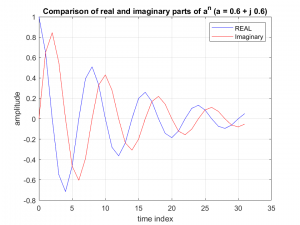
Figure 3.3 Sequence for aⁿ Where a is Complex.

It should be noted that the oscillatory nature of the sequence is very similar to the dying exponentials that are commonly the solution to a linear circuits impulse response.  In fact if we take the response of a linear system [latex]e^{(\alpha + j \omega) t ) [/latex] and replace t with n T, we have

[latex]e^{(\alpha + j \omega) n T }  = (e^{ ( \alpha + j \omega ) T } )^n[/latex]                 (3.17)

And these are equivalent if

[latex]a = e^{(\alpha + j \omega) T }[/latex]                                                                          (3.18)

Recall that previously we stated that |a| < 1 for the z transform to converge.  This will relate to the stability of the system.  Consider the absolute value of 3.18

[latex]| a | = | e^{(\alpha + j \omega) T )} | = | e^{\alpha T} * e^{j \omega) T} |[/latex]                 (3.19)

$latex              = | e^{\alpha T} | * |  e^{j \omega) T )} | $                                                                          (3.20)

Now since [latex]|  e^{j \omega) T } = 1[/latex] we can see that

[latex]| a | = | e^{\alpha T} |[/latex]                                          (3.21)

And as long as alpha is negative, we will have a dying exponential and |a| < 1.

For this reason, the unit circle in the complex plane will play an important role in much of the analysis of the z transform.  The following video is meant as a visual or intuitive demonstration of this principle.

In the next section we will explore more about how to visualize and apply z transforms.

Section B) The z Transform of a Delayed sequence.

We begin by considering the effect of delaying the sampled sequence by one sample.  We will first note that the z transform is a summation and looks like

[latex]\sum_{n=0} ^{\infty} (  x(n)  * z^{-n}  )  = x(0)  + x(1) z^{-1} + x(2) z^{-2} + x(3) z^{-3} + ...[/latex]           (3.22)

Note the … indicates that the sequence continues on in the manner shown.  The z transform of the delayed version, x(n-1), is then

[latex]\hat X(z) = \sum_{n=0} ^{\infty} x(n-1) z^{-n}[/latex]   (3.23)

Writing out the summation we would have

[latex]\hat X(z) =  x(-1) + x(0) z^{-1} + x(1) z^{-2} + x(2) z^{-3} + ...[/latex]   (3.24)

Next we set out x(-1) and factor out a single [latex]z^{-1}[/latex] from the remainder.

[latex]\hat X(z) = x(-1) + z^{-1} ( x(0) + x(1) z^{-1} + x(2) z^{-2} + ... )[/latex]         (3.25)

We can now observe that sum on the right, in parenthesis, is the z transform of x(n) or X(z) and thus

[latex]\hat X(z) = x(-1) + z^{-1}  X(z) [/latex]                                                 (3.26)

This property is analogous to the Laplace transform of the derivative of a function, and points to the Difference Equations (DE) that we will use to process discrete data.

Section C) z Transform to Frequency Response

One of the primary approaches used to analyze systems and data is its frequency response.  So how might we go from the z transform to a frequency response?  We start by looking at sampled cosine and applying the Euler identity for a cosine we have

[latex]x(n) = cos( \omega_o n T) = \frac{1}{2} ( e^{j \omega_o n T} + e^{- j \omega_o n T})[/latex]       (3.27)

Factoring 3.27 we have

[latex]x(n) = \frac{1}{2} ( (e^{j \omega_o T} )^n + (e^{- j \omega_o T})^n )[/latex]                       (3.28)

Looking close at 3.28, we can see that it has the form of two sequences of the form [latex]a^n[/latex], where [latex]a = e^{\pm j \omega_o T}[/latex]. Thus the z transform of the signal would  be

[latex]X(z) = \frac{1}{2} ( \frac{1}{1 - z^{-1} e^{j \omega_o T}} + \frac{1}{1 - z^{-1} e^{- j \omega_o T}} )[/latex]            (3.29)

Thus the z transform would have two poles, at [latex]z = e^{\pm j \omega_o T}[/latex].  To make this more understandable, we convert to frequencies by [latex]\omega_o = 2 \pi f_o[/latex] and [latex]T = \frac{1}{f_s}[/latex] which will become

[latex]X(z) = \frac{1}{2} ( \frac{1}{1 - z^{-1} e^{j 2 \pi \frac{f_o}{f_s}}} + \frac{1}{1 - z^{-1} e^{- j 2 \pi \frac{f_o}{f_s}}} )[/latex]            (3.30)

Another way to view this is to plot the location of the poles (z values where X(z) = [latex]\infty[/latex]) whichi is at [latex]z = e^{\pm j 2 \pi \frac{f_o}{f_s}}[/latex] which is what the following video will display.

The prime thing to take away from this section is the fact that the z transform at the unit circle, represents the frequency response of the system.

Section D.1) The z Transform of a Difference Equation

A difference equation will be the primary form used to process the discrete data.  A basic, second order, example is shown here

[latex]y(n) = b_0 x(n) + b_1 x(n-1) + b_2 x(n-2) - a_1 y(n-1) - a_2 y(n-2)       [/latex]                      (3.27)

The basic structure of this equations is that we create an output sequence, y(n), by computing a weighted average of current and past inputs (x(n), x(n-1) & x(n-2)) and past outputs (y(n-1) & y(n-2)).

If we take the z transform of 3.22 we would have

[latex]Y(z) = b_0 X(z) + b_1(x(-1) + z^{-1} X(z)) + b_2 (x(-2) + z^{-1} x(-1) + z^{-2} X(z)) - a_1 (y(-1) + z^{-1} Y(z)) - e (y(-2) + z^{-1} y(-1) + z^{-2} Y(z)) [/latex]                                                     (3.28)

It should be noted that we have applied the property in 3.21, recursively in this equation to find the z transform of x(n-2), as in

[latex]Z\{ x(n-2) \} = x(-2) + z * Z\{ x(n-1)\} = x(-2) + z^{-1} ( x(-1) + z X(z)) = x(-2) + z^{-1} x(-1) + z^{-2} X(z) [/latex]             (3.29)

where Z{x(n)} is the z transform of x(n) or X(z).

Since the primary goal is to solve for the output, y(n), we will now solve 3.23 by first moving all the Y(z)’s to the Left Hand Side (LHS) and reordering with like terms on the Right Hand Side (RHS).

[latex]Y(z) + d z^{-1} Y(z) + e z^{-2} Y(z) = b_0 X(z) + b_1 z^{-1} X(z) + b_2 z^{-2} X(z) + (b_1 + b_2 z^{-1}) x(-1) + b_2 x(-2 ) - (a_1 + a_2 z^{-1}) y(-1) - a_2 y(-2)[/latex]                                 (3.30)

Factoring our the Y(z) on the left hand side and similar approach for X(z) we have

[latex]Y(z) (1 + d z^{-1} + e z^{-2}) = X(z) ( b_0 + b_1 z^{-1}+ b_2 z^{-2} ) + (b_1 + b_2 z^{-1}) x(-1) + b_2 x(-2 ) - (a_1 + a_2 z^{-1}) y(-1) - a_2 y(-2)[/latex]       (3.31)

Dividing both sides by [latex](1 + d z^{-1} + e z^{-2})[/latex] yields

[latex]Y(z)  = X(z) \frac{( b_0 + b_1 z^{-1}+ b_2 z^{-2} )}{(1 + a_1 z^{-1} + a_2 z^{-2})} + x(-1) \frac{(b_1 + b_2z^{-1})}{(1 + a_1 z^{-1} + a_2 z^{-2})} + x(-2 ) \frac{b_2}{(1 + a_1 z^{-1} + a_2 z^{-2})} - y(-1) \frac{(a_1 + a_2 z^{-1})}{(1 + a_1 z^{-1} + a_2 z^{-2})} - y(-2) \frac{a_2}{(1 + a_1 z^{-1} + a_2 z^{-2})}[/latex]                                (3.32)

Now if we were to insert X(z) (based on our input) and values for x(-1), x(-2), y(-1) and y(-2) we could merge all the terms on the RHS into a rational function that can be inverse transformed to the sequence y(n).  This solution is however, little more than an academic exercise and we will walk through it in a later example.  However a more common application and use will be use the Y(z) to X(z) relationship to understand the effect of the difference equation.  To describe this relationship a common thing to do is set the initial conditions to zero.  This results in the classic form of

[latex]Y(z)  = X(z) \frac{( b_0 + b_1 z^{-1}+ b_2 z^{-2} )}{(1 + a_1 z^{-1} + a_2 z^{-2})} [/latex]                                (3.33)

or

[latex]Y(z)  = X(z) H(z)[/latex]                                                                                      (3.34)

where H(z) is known as the transfer function.

Section D.2) Example of difference equation using z transforms.

Consider the DE below

[latex]y(n) = 0.25 x(n) + 0.5 x(n-1) + 0.25 x(n-2) + y(n-1) - 0.5 y(n-2)[/latex]                                           (3.35)

Taking the z transform of this DE and factoring it similarly to was done previously, we have

[latex]Y(z)  = X(z) \frac{( 0.25 + 0.5  z^{-1}+ 0.25 z^{-2} )}{(1 - z^{-1} + 0.5 z^{-2})} [/latex]                                (3.36)

or

[latex]H(z) = \frac{( 0.25 + 0.5  z^{-1}+ 0.25 z^{-2} )}{(1 - z^{-1} + 0.5 z^{-2})} [/latex]                                (3.37)

As an added point, note the change in sign on the denominator between 3.35 and 3.36/3.37

The following video will show how we can visualize and interpret the z-transform transfer function and its effect on a signal.

MATLAB Code from Video

Section E.1) Graphical Representation of Difference Equations

In this section we will be discussing a graphical representation of a difference equation (DE).  Although at first this may appear to not be that important, but as we develop our understanding of DE’s we will find this representation is quite powerful.  In Figure 3.4 we can see the basic building blocks for describing a DE.

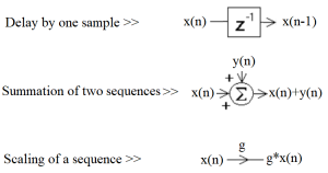
Figure 3.4  Basic Building Blocks for Graphically Representing Difference Equations.

Rather than walking through some type of generic process for developing these graphical descriptions, commonly called Signal Flow Diagrams (SFD), it is believed that an example is more instructive.  For this we will implement the following simple first-order DE.

[latex]y(n) = x(n) + x(n-1) +  0.75 y(n-1)[/latex]                                           (3.38)

We start with a delay of the input x(n) as shown in Figure 3.5.

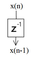
Figure 3.5 First Part of DE

Conceptually we can look at the [latex]z^{-1}[/latex] element as a register that holds the value of x(n) and thus delays it by one sample.  We can now take the two version of the input we have (x(n) and x(n-1)) and add them together as in Figure 3.6.

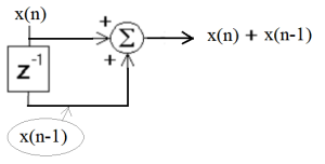
Figure 3.6 Implementation of The “Feed Forward” Portion of The DE.

Again the summation element is simply an adder that takes the current input value on each line and adds them together.  Also it should be noted that this portion of the system was called “Feed Forward”, since it only uses the inputs, which are feed from the input forward towards the output.

If you now add in the feed back portion of the DE, by delaying the output y(n), scaling it by 0.75 and adding it with the feed forward portion from Figure 3.6.

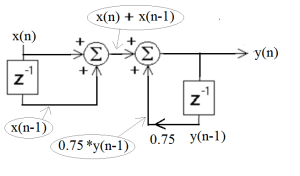
Figure 3.7 Full Implementation of Difference Equation.

At this point we have a SFD of the DE in equation 3.38.  It is important to note that the equations inserted and circled in gray are meant to clarify the process and are not commonly added to the signal graph.

Section E.2) Example of How A Signal Flow Graph Can Be Used.

Consider the DE in equation 3.27 (replicated here).  This second order DE will be a standard building block for many of the filters we design.

[latex]y(n) = b_0 x(n) + b_1 x(n-1) + b_2 x(n-2) - a_1 y(n-1) - a_2 y(n-2)       [/latex]                      (3.27)

Following the process used for the first-order DE above we can create the SFD shown in Figure 3.8

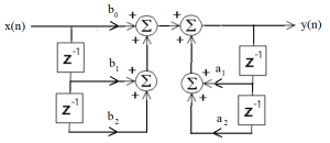
Figure 3.8 Second Order DE As a Signal Flow Diagram

This form of implementation is known as a Direct Form I, as it follows the DE in a “direct” fashion.  Now since the feed forward and feedback sections are independent, they can be reordered as shown in Figure 3.9.

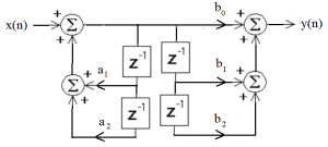
Figure 3.9 Signal Flow Graph With Sections Reordered.

Now this form is not that different from the Direct Form I.  However, since the delay elements are actually delaying the same signal they can be merged as shown in 3.10.

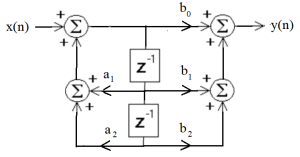
Figure 3.10 Signal Flow Graph With Delay Elements Merged.

This has an advantage that only two delay elements (or memory locations) are used and defined as a Direct Form II.  Although that is of some help, there are other changes that can be used on a SFD.  We will not work through these techniques, however specialists in system theory have developed what is know as a transposed form for an SFD.

The rules for converting to a transposed form are rather esoteric and can be confusing, suffice it to say the input and output are switched, the direction on the components in the SFD are all changed and junctions are replaced with summations and vice versa.  The result is shown in Figure 3.11.

Figure 3.11 Transposed Signal Flow Diagram.

Now this form is actually helpful when implementing the system.  However, in order to validate that it implements the second-order DE we will walk through the various parts of the process.  These are laid out in Figure 3.12.

In 3.12, we can see that we start at the bottom, x(n) and y(n) are scaled by [latex]a_2[/latex] & [latex]b_2[/latex] and then added together (Eq 1).  That sum is then delayed through the bottom [latex]z^{-1}[/latex] component (Eq 2).  The next level up will take x(n) and y(n), scaled by [latex]a_1[/latex] & [latex]b_1[/latex] and add them to the previous sum (Eq 3).  That sum is then delayed through the bottom [latex]z^{-1}[/latex] component (Eq 4).  Finally, x(n) is multiplied by [latex]b_0[/latex] and added in, arriving at final equation (Eq 5), which is the DE were were working to implement.

Figure 3.12 Transposed Signal Flow Graph With Intermediate Signals Annotated.

Section E.3) Effect On Code of The Direct and Transposed Forms.

Having described and validated these implementation forms for the DE’s, the questions is “What does that help us?”  In order to address that, two version of code that will implement a second order system using the Direct Form I and the Transposed Direct Form II.

The first box here shows the code for the Direct Form I.  The basic structure of the code is a c function that is called as each sample ( x ) comes in.  It then computes the next output ( y ), based on the current input and the delayed copies of the input and output.  The most notable part of this code is that the output y is computed with 5 Multiply and ADD’s (MADD’s), then a four lines of code are used to implement the delays need in preparation for the next call of the function.   This extra step is one of the challenges with this form of implementation.

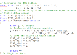
Of these two approaches, the transposed form is often considered the preferred method for implementing a second order system.

Section F) Conclusion

In this chapter we have established the format and uses of the z-transform, showing various ways we can visualize and interpret the z-transform.  Perhaps the most important feature is how it relates to the DE, our primary way of processing data, and its relationship to the frequency response of a DE.

In the next chapter we will be looking at ways we can design a filter, using two basic forms.  The first is the Finite Impulse Response (FIR) filter, or a feed forward filter, and the second uses feedback and has an Infinite Impulse Response (IIR).