Main Body
Chapter 7. Game Theory Applications
7.1 Repeated and Sequential Games
7.1.1 Repeated Games
A game that is played only once is called a “one-shot” game. Repeated games are games that are played over and over again.
Repeated Game = A game in which actions are taken and payoffs received over and over again.
Many oligopolists and real-life relationships can be characterized as a repeated game. Strategies in a repeated game are often more complex than strategies in a one-shot game, as the players need to be concerned about the reactions and potential retaliations of other players. As such, the players in repeated games are likely to choose cooperative or “win-win” strategies more often than in one shot games. Examples include concealed carry gun permits: are you more likely to start a fight in a no-gun establishment, or one that allows concealed carry guns? Franchises such as McDonalds were established to allow consumers to get a common product and consistent quality at locations new to them. This allows consumers to choose a product that they know will be the same, given the repeated game nature of the decision to purchase meals at McDonalds.
7.1.2 Sequential Games
A sequential game is played in “turns,” or “rounds” like chess or checkers, where each player takes a turn.
Sequential Game = A game in which players move in turns, responding to each others’ actions and reactions.
7.1.3 Product Choice Game One
An example of a sequential game is the product choice game shown in Figure 7.1.
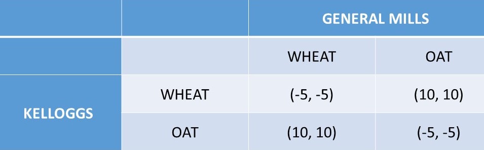
Figure 7.1 Product Choice Game One: Cereal. Outcomes are in million USD.
In this game, two cereal producers (Kelloggs and General Mills) decide whether to produce and sell cereal made from wheat or oats. If both firms select the same category, both firms lose five million USD, since they have flooded the market with too much cereal. However, the two firms split the two markets, with one firm producing wheat cereal and the other firm producing oat cereal, both firms earn ten million USD. In this situation, it helps both firms if they can decide which firm goes first, to signal to the other firm. It does not matter which firm produces wheat or oat cereal, as long as the two firms divide the two markets. This type of repeated game can be solved by one firm going first, or signaling to the other firm which product it will produce, and letting the other firm take the other market.
7.1.4 Product Choice Game Two
It might be that one of the two markets is more valuable than the other. This situation is shown in Figure 7.2.
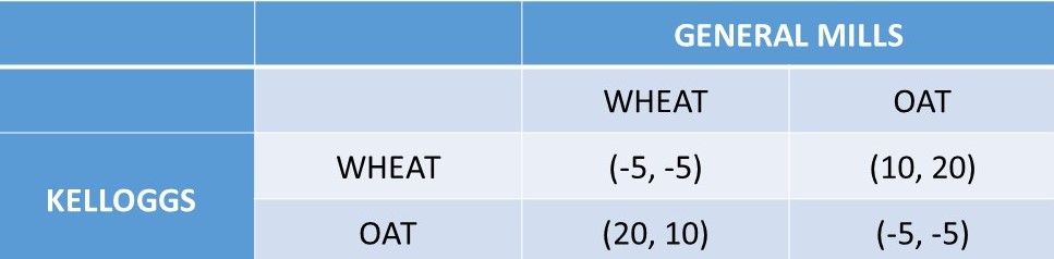
Figure 7.2 Product Choice Game Two: Cereal. Outcomes are in million USD.
This cereal market game is very similar to the previous game, but in this case the oat cereal market is worth much more than the wheat cereal market. As in the Product Choice One game, if both firms select the same market, both lose five million USD. Similarly, if each firm chooses a different market, then both firms make positive economic profits. The difference between the two product choice games is that the earnings are asymmetrical in the Product Choice Two game (Figure 7.2): the firm that is in the oat cereal market earns 20 million USD, and the firm in the wheat cereal market earns 10 million USD. In this situation, both firms will want to choose OAT first. If Kelloggs is able to choose OAT first, then it is in General Mill’s best interest to select WHEAT. The player in this sequential game who goes first has a first player advantage, worth ten million USD. Each firm would be willing to pay up to ten million USD for the right to select first. In a repeated game, the market stabilizes with one firm producing oat cereal, and the other firm producing wheat cereal. There is no advantage for either firm to switch strategies, unless the firm can play OAT first, causing the other firm to move into wheat cereal.
7.2 First Mover Advantage
The first mover advantage is similar to the Stackelberg model of oligopoly, where the leader firm had an advantage over the follower firm. In many oligopoly situations, it pays to go first by entering a market before other firms. In many situations, it pays to determine the firm’s level of output first, before other firms in the industry can decide how much to produce. Game theory demonstrates how many real-world firms determine their output levels in an oligopoly.
7.2.1 First Mover Advantage Example: Ethanol
Ethanol provides a good example of the first-mover advantage. Consider an ethanol market that is a Stackelberg duopoly. To review the Stackelberg model, assume that there are two ethanol firms in the same market, and the inverse demand for ethanol is given by P = 120 – 2Q, where P is the price of ethanol in USD/gallon, and Q is the quantity of ethanol in million gallons. The cost of producing ethanol is given by C(Q) = 12Q, and total output is the sum of the two individual firm outputs: Q = Q1 + Q2.
First, suppose that the two firms are identical, and they are Cournot duopolists. To solve this model, Firm One maximizes profits:
max π1 = TR1 – TC1
max π1 = P(Q)Q1 – C(Q1)[price depends on total output Q = Q1 + Q2]
max π1 = [120 – 2Q]Q1 – 12Q1
max π1 = [120 – 2Q1 – 2Q2]Q1 – 12Q1
max π1 = 120Q1 – 2Q12 – 2Q2Q1 – 12Q1
∂π1/∂Q1= 120 – 4Q1 – 2Q2 – 12 = 0
4Q1 = 108 – 2Q2
Q1* = 27 – 0.5Q2 million gallons of ethanol
This is Firm One’s reaction function. Assuming identical firms, by symmetry:
Q2* = 27 – 0.5Q1
The solution is found through substitution of one equation into the other.
Q1* = 27 – 0.5(27 – 0.5Q1)
Q1* = 27 – 13.5 + 0.25Q1
Q1* = 13.5 + 0.25Q1
0.75Q1* = 13.5
Q1* = 18 million gallons of ethanol
Due to symmetry from the assumption of identical firms:
Qi = 18 million gallons of ethanol, i = 1,2
Q = 36million gallons of ethanol
P = 48 USD/gallon ethanol
Profits for each firm are:
πi = P(Q)Qi – C(Qi) = 48(18) – 12(18) = (48 – 12)18 = 36(18) = 648 million USD
This result shows that if each firm produces 18 million gallons of ethanol, each firm will earn 648 million USD in profits. This is shown in Figure 7.3, where several different possible output levels are shown as strategies for Firm A and Firm B, together with payoffs.
Next, suppose that the two firms are not identical, and that one firm is a leader and the other is the follower. By calculating the Stackelberg model solution, the possible outcomes of the game can be derived, as shown in Figure 7.3.
In the Stackelberg model, assume that Firm One is the leader and Firm Two is the follower. In this case, Firm One solves for Firm Two’s reaction function:
max π2 = TR2 – TC2
max π2 = P(Q)Q2 – C(Q2)[price depends on total output Q = Q1 + Q2]
max π2 = [120 – 2Q]Q2 – 12Q2
max π2 = [120 – 2Q1 – 2Q2]Q2 – 12Q2
max π2 = 120Q2 – 2Q1Q2 – 2Q22 – 12Q2
∂π2/∂Q2= 120 – 2Q1 – 4Q2 – 12 = 0
4Q2 = 108 – 2Q1
Q2* = 27 – 0.5Q1
Next, Firm One, the leader, maximizes profits holding the follower’s output constant using the reaction function:
max π1 = TR1 – TC1
max π1 = P(Q)Q1 – C(Q1)[price depends on total output Q = Q1 + Q2]
max π1 = [120 – 2Q]Q1 – 12Q1
max π1 = [120 – 2Q1 – 2Q2]Q1 – 12Q1
max π1 = [120 – 2Q1 – 2(27 – 0.5Q1)]Q1 – 12Q1 [substitution of One’s reaction function]
max π1 = [120 – 2Q1 – 54 + Q1]Q1 – 12Q1
max π1 = [66 – Q1]Q1 – 12Q1
max π1 = 66Q1 – Q12 – 12Q1
∂π1/∂Q1= 66 – 2Q1 – 12 = 0
2Q1* = 54
Q1* = 27 million gallons of ethanol
This can be substituted back into Firm Two’s reaction function to solve for Q2*.
Q2* = 27 – 0.5Q1 = 27 – 0.5(27) = 27 – 13.5 = 13.5 million gallons of ethanol
Q = Q1 + Q2 = 27 + 13.5 = 40.5 million gallons of ethanol
P = 120 – 2Q = 120 – 2(40.5) = 120 – 81 = 39 USD/gallon ethanol
π1 = (39 – 12)27 = 27(27) = 729 million USD
π2 = (39 – 12)13.5 = 27(13.5) = 364.5 million USD
These results are displayed in Figure 7.3. In a one-shot game, the Nash Equilibrium is (18, 18), yielding payoffs of 648 million USD for each ethanol plant in the market. Each firm desires to select 18 million gallons, and have the other firm select 13.5 million gallons, in which case profits would increase to 810 million USD. However, the rival firm will not unilaterally cut production to 13.5, since it would lose profits at the expense of the other firm.
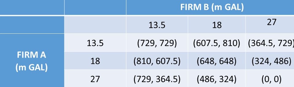
Figure 7.3 First-Mover Advantage: Ethanol. Outcomes are in million USD.
In a sequential game, if Firm A goes first, it will select 27 million gallons of ethanol. In this case, Firm B will choose to produce 13.5 million gallons of ethanol, which is the Stackelberg solution. Firm A, as the first mover, has increased profits from 648 to 729 million USD by being able to go first. This is the first mover advantage.
7.2.2 Empty Threat
Figure 7.4 shows a sequential game between two grain seed dealers: Monsanto, a large international agribusiness, and a Local Grower. Monsanto is the dominant firm, and chooses a pricing strategy first. If Monsanto selects a HIGH price strategy, the Local Grower will select a LOW price, and both firms are profitable. In this case, the Local Grower has the low price, so makes more money than Monsanto.
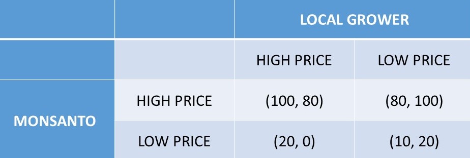
Figure 7.4 Empty Threat: Grain Seed Dealers. Outcomes are in million USD.
Could Monsanto threaten the Local Grower that it would set a LOW price, to try to cause the Local Grower to set a HIGH price, and increasing Monsanto profits from 80 million USD to 100 million USD? Monsanto could threaten to set a LOW price, but it is not believable, since Monsanto would have very low payoffs in both outcomes. In this case, Monsanto’s threat is an empty threat, since it is neither credible nor believable.
7.2.3 Pre-Emptive Strike
Suppose two big box stores are considering entering a small town market. If both Walmart and Target enter this market, both firms lose ten million USD, since the town is not large enough to support both firms. However, if one firm can enter the market first (a “pre-emptive strike”), it can gain the entire market and earn 20 million USD. The firm that goes first wins this game in a significant way. This explains why Walmart has opened so many stores in a large number of small cities.

Figure 7.5 Pre-Emptive Strike: Big Box Stores. Outcomes are in million USD.
7.2.4 Commitment and Credibility
Figure 7.6 shows a sequential game between beef producers and beef packers. In this game, the packer is the leader, and decides to produce and sell LOW or HIGH quality beef.
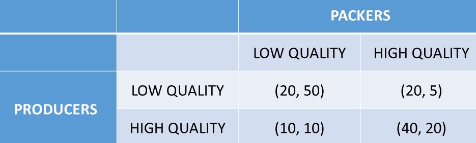
Figure 7.6 Commitment and Credibility One: Beef Industry. Outcomes are in m USD.
If the packers go first, they will select LOW, since they know that by doing so, the producers would also select LOW. This results in 50 million USD for the packers and 20 million USD for the producers. The producers would prefer the outcome (HIGH, HIGH), as their profits would increase from 20 to 40 million USD. In this situation, the beef producers can threaten the packers by committing to producing HIGH quality beef only. The packers will select LOW if they do not believe the threat, in the attempt to achieve the outcome (LOW, LOW). However, if the producers can commit to the HIGH quality strategy, and prove to the packers that they will definitely choose HIGH quality, the packers would choose HIGH also, and the producers would achieve 40 million USD.
The producers could come up with a strategy of visibly and irreversibly reducing their own payoffs to prove to the packers that they are serious about HIGH quality, and cause the packers to choose HIGH also. This commitment, if credible, could change the outcome of the game, resulting in higher profits for the producers, at the expense of the packers. Such a credible commitment is shown in Figure 7.7, which replicates Figure 7.6 with the exception of the LOW outcomes for the producers. If the beef producers sell off their low quality herd, and have no low quality cattle, they change the sequential game from the one shown in Figure 6.9 to the one in Figure 6.10.
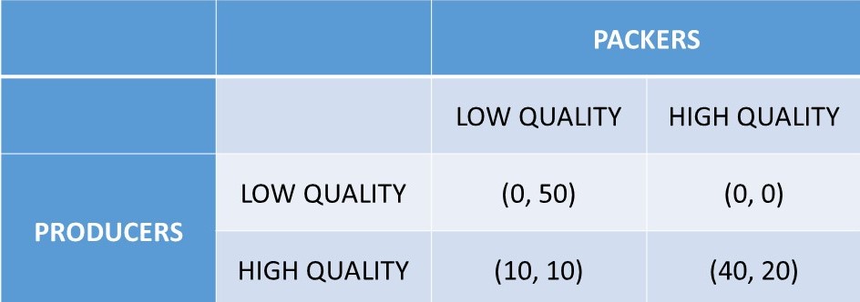
Figure 7.7 Commitment and Credibility Two: Beef Industry. Outcomes are in m USD.
If the packers are the leaders in Figure 7.7, they select the HIGH quality strategy. If they select LOW, the producers would choose HIGH, yielding 10 million USD for the packers. When the packers select HIGH, the packers earn 20 million USD. Therefore, a producer strategy of shutting down or destroying the low quality productive capacity results in the desired outcome for the producers: (HIGH, HIGH). The strategy of taking an action that appears to put a firm at a disadvantage can provide the incentives to increase the payoffs of a sequential game. This strategy can be effective, but is risky. The producers need accurate knowledge of the payoffs of each strategy.
The commitment and credibility game is related to barriers to entry in monopoly. A monopolist often has a strong incentive to keep other firms out of the market. The monopolist will engage in entry deterrence by making a credible threat of price warfare to deter entry of other firms. In many situations, a player who behaves irrationally and belligerently can keep rivals off balance, and change the outcome of a game. Political leaders who appear irrational may be using their unpredictability to achieve long run goals.
A policy example of this type of strategy occurs during bargaining between politicians. If one issue is not going in a desired direction, a political group can bring in another issue to attempt to persuade the other party to compromise.
The “holdup game” is another example of commitment and credibility. Often, once significant resources are committed to a project, the investor will ask for more resources. If the project is incomplete, the funder will often agree to pay more money to have the project completed. Large building projects are often subject to the holdup game.
For example, if a contractor has been paid 20 million USD to build a campus building, and the project is only 50 percent complete, the contractor could halt construction, letting the half-way completed building sit unfinished, and ask for 10 million USD more, due to “cost overruns.” This strategy is often effective, even if a contract is carefully and legally drawn up ahead of time. The contractor has the University right where they want it: stuck with an unfinished building unless they increase the dollars to the project. The contractor is effectively saying, “do it my way, or I quit.”
