Main Body
Chapter 3. Monopoly and Market Power
3.1 Market Power Introduction
This chapter will explore firms that have market power, or the ability to set the price of the good that they produce.
Market Power = Ability of a firm to set the price of a good. Also called monopoly power.
A monopoly is defined as a single firm in an industry with no close substitutes. An industry is defined as a group of firms that produce the same good.
Monopoly = A single firm in an industry with no close substitutes.
The phrase, “no close substitutes” is important, since there are many firms that are the sole producer of a good. Consider McDonalds Big Mac hamburgers. McDonalds is the only provider of Big Macs, yet it is not a monopoly because there are many close substitutes available: Burger King Whoppers, for example.
Market power is also called monopoly power. A competitive firm is a “price taker.” Thus, a competitive firm has no ability to change the price of a good. Each competitive firm is small relative to the market, so has no influence on price. On the other hand, firms with market power are also called “price makers.”
Price Taker = A competitive firm with no ability to set the price of a good.
Price Maker = A noncompetitive firm with market power, defined as the ability to set the price of a good.
A monopolist is considered to be a price maker, and can set the price of the product that it sells. However, the monopolist is constrained by consumer willingness and ability to purchase the good, also called demand. For example, suppose that an agricultural chemical firm has a patent for an agricultural chemical used to kill weeds, a herbicide. The patent is a legal restriction that permits the patent holder to be the only seller of the herbicide, as it was invented by the company through their research program. In Figure 3.1, an agricultural chemical firm faces an inverse demand curve equal to: P = 100 – Qd, where P is the price of the agricultural chemical in dollars per ounce (USD/oz), and Qd is the quantity demanded of the chemical in million ounces (m oz).
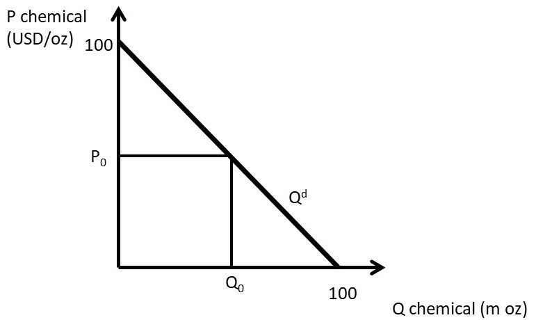
Figure 3.1 Demand Facing a Monopolist: Agricultural Chemical
The monopolist can set a price, but the resulting quantity is determined by the consumers’ willingness to pay, or the demand curve. For example, if the price is set at P0, consumers will purchase Q0. Alternatively, the monopolist could set quantity at Q0, and consumers would be willing to pay P0 for Q0 units of the chemical. Thus, a monopolist has the ability to set any price that it would like to, but with important limitation: the monopolist is constrained by consumer willingness to pay for the product.
3.2 Monopoly Profit-Maximizing Solution
The profit-maximizing solution for the monopolist is found by locating the biggest difference between total revenues (TR) and total costs (TC), as in Equation 3.1.
(3.1) max π = TR – TC
3.2.1 Monopoly Revenues
Revenues are the money that a firm receives from the sale of a product.
Total Revenue [TR] = The amount of money received when the producer sells the product. TR = PQ
Average Revenue [AR] = The average dollar amount receive per unit of output sold AR = TR/Q
Marginal Revenue [MR] = the addition to total revenue from selling one more unit of output.
MR = ΔTR/ΔQ = ∂TR/∂Q.
TR = PQ (USD)
AR = TR/Q = P(USD/unit)
MR = ΔTR/ΔQ = ∂TR/∂Q (USD/unit)
For the agricultural chemical company:
TR = PQ = (100 – Q)Q = 100Q – Q2
AR = P = 100 – Q
MR = ∂TR/∂Q = 100 – 2Q
Total revenues for the monopolist are shown in Figure 3.2. Total Revenues are in the shape of an inverted parabola. The maximum value can be found by taking the first derivative of TR, and setting it equal to zero. The first derivative of TR is the slope of the TR function, and when it is equal to zero, the slope is equal to zero.
(3.2) max TR = PQ ∂TR/∂Q = 100 – 2Q = 0 Q* = 50
Substitution of Q* back into the TR function yields TR = USD 2500, the maximum level of total revenues (Figure 3.2).
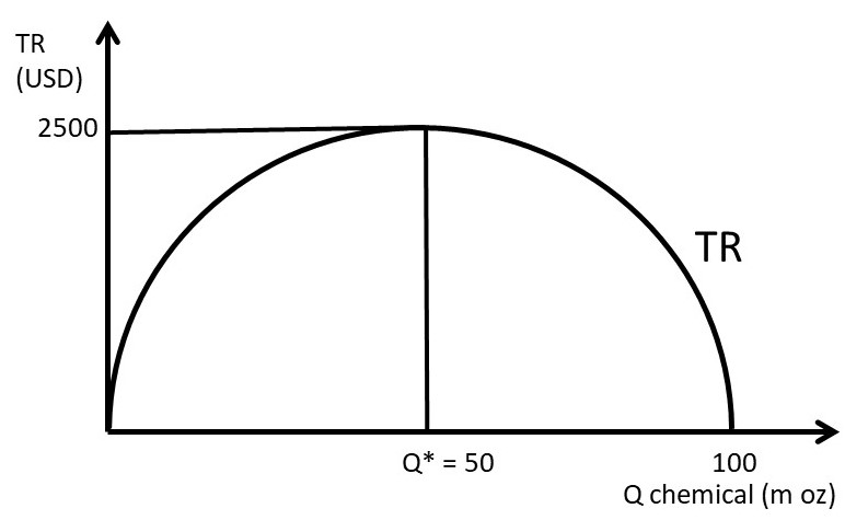
Figure 3.2 Total Revenues for a Monopolist: Agricultural Chemical
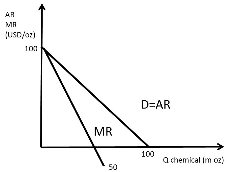
Figure 3.3 Per-Unit Revenues for a Monopolist: Agricultural Chemical
It is important to point out that the optimal level of chemical is not this level. The optimal level of chemical to produce and sell is the profit-maximizing level, which is revenues minus costs. If the monopolist were to maximize revenues instead of profits, it might cost too much relative to the gain in revenue. Profits include both revenues and costs.
Average revenue (AR) and marginal revenue (MR) are shown in Figure 3.3. The marginal revenue curve has the same y-intercept and twice the slope as the average revenue curve. This is always true for linear demand (average revenue) curves. This is one of the major take home messages of economics: maximize revenues may cost too much to make it worth it. For example, a corn farmer who maximizes yield (output per acre of land) may be spending too much on inputs such as fertilizer and chemicals make the higher yield payoff. From an economic perspective, the corn farmer should consider both revenues and costs.
3.2.2 Monopoly Costs
The costs for the chemical include total, average, and marginal costs.
Total Cost [TC] = The sum of all payments that a firm must make to purchase the factors of production. The sum of Total Fixed Costs and Total Variable Costs. TC = C(Q) = TFC + TVC.
Total Fixed Costs [TFC] = Costs that do not vary with the level of output.
Total Variable Costs [TVC] = Costs that do vary with the level of output.
Average Cost [AC] = total costs per unit of output. AC = TC/Q. Note that the terms, Average Costs and Average Total Costs are interchangeable.
Marginal Cost [MC] = the increase in total costs due to the production of one more unit of output. MC = ΔTC/ΔQ = ∂TC/∂Q.
TC = C(Q)(USD)
AC = TC/Q(USD/unit)
MC = ΔTC/ΔQ = ∂TC/∂Q (USD/unit)
Suppose that the agricultural chemical firm is a constant cost industry. This means that the per-unit cost of producing one more ounce of chemical is the same, no matter what quantity is produced. Assume that the cost per unit is ten dollars per ounce (10 USD/oz).
TC = 10Q
AC = TC/Q = 10
MC = ΔTC/ΔQ = ∂TC/∂Q = 10
The total costs are shown in Figure 3.4, and the per-unit costs are in Figure 3.5.
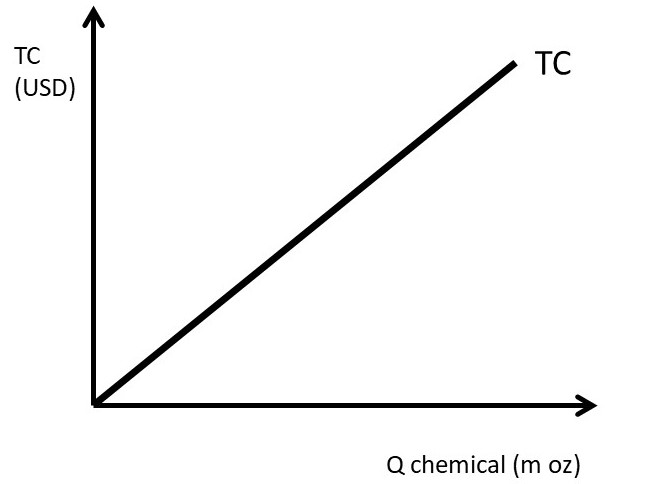
Figure 3.4 Total Costs for a Monopolist: Agricultural Chemical
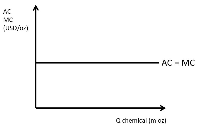
Figure 3.5 Per-Unit Costs for a Monopolist: Agricultural Chemical
3.2.3 Monopoly Profit-Maximizing Solution
There are three ways to communicate economics: verbally, graphically, and mathematically. The firm’s profit maximizing solution is one of the major features and important conclusions of economics. The verbal explanation is that a firm should continue any activity as long as the additional (marginal) benefits are greater than the additional (marginal) costs. The firm should continue the activity until the marginal benefit is equal to the marginal cost. This is true for any activity, and for profit maximization, the firm will find the optimal, profit maximizing level of output where marginal revenues equal marginal costs (MR = MC).
The graphical solution takes advantage of pictures that tell the same story, as in Figures 3.6 and 3.7. Figure 3.6 shows the profit maximizing solution using total revenues and total costs. The profit-maximizing level of output is found where the distance between TR and TC is largest: π = TR – TC. The solution is found by setting the slope of TR equal to the slope of TC: this is where the rates of change are equal to each other (MR = MC).
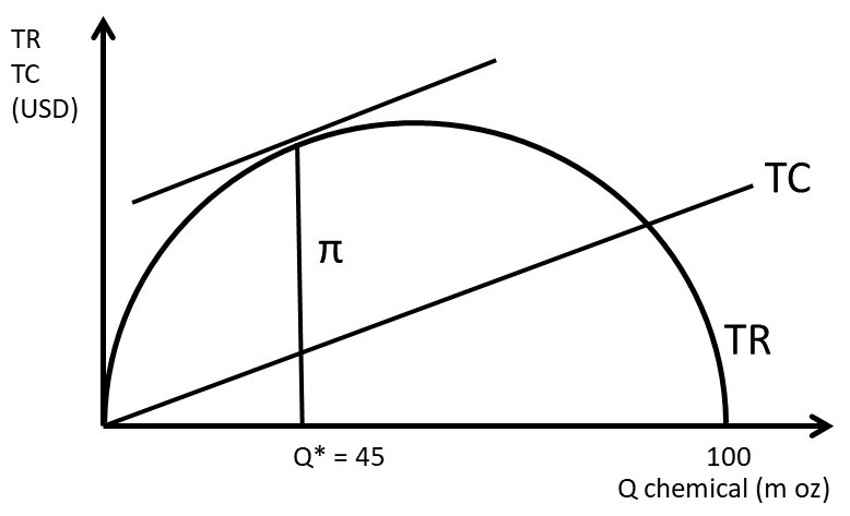
Figure 3.6 Total Profit Solution for a Monopolist: Agricultural Chemical
The same solution can be found using the marginal graph (Figure 3.7). The firm sets MR equal to MC to find the profit-maximizing level of output (Q*), then substitutes Q* into the consumers’ willingness to pay (demand curve) to find the optimal price (P*). The profit level is an area in Figure 3.7, defined by TR and TC. Total revenues are equal to price times quantity (TR = P*Q), so TR are equal to the rectangle from the origin to P* and Q*. Total costs are equal to the rectangle defined by the per-unit cost of ten dollars per ounce times the quantity produced, Q*. If the TC rectangle is subtracted from the TR rectangle, the shaded profit rectangle remains: profits are the residual of revenues after all costs have been paid (π = TR – TC).
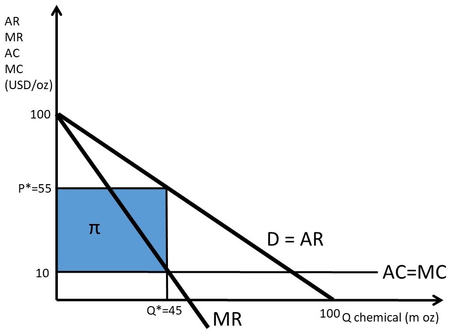
Figure 3.7 Marginal Profit Solution for a Monopolist: Agricultural Chemical
The math solution for profit maximization is found by using calculus. The maximum level of a function is found by taking the first derivative and setting it equal to zero. Recall that the inverse demand function facing the monopolist is P = 100 – Qd, and the per unit costs are ten dollars per ounce.
max π = TR – TC
= P(Q)Q – C(Q)
= (100 – Q)Q – 10Q
= 100Q – Q2 – 10Q
∂π/∂Q= 100 – 2Q – 10 = 0
2Q = 90
Q* = 45 million ounces of agricultural chemical
The profit-maximizing price is found by substituting Q* into the inverse demand equation:
P* = 100 – Q* = 100 – 45 = 55 USD/ounce of agricultural chemical.
The maximum profit level can be found by substitution of P* and Q* into the profit equation:
π = TR – TC = P(Q)Q – C(Q) = 55*45 – 10*45 = 45*45 = 2025 million USD.
This profit level is equal to the distance between the TR and TC curves at Q* in Figure 3.6, and the profit rectangle identified in Figure 3.7. The profit-maximizing level of output and price have been found in three ways: verbally, graphically, and mathematically.
3.3 Marginal Revenue and the Elasticity of Demand
We have located the profit-maximizing level of output and price for a monopoly. How does the monopolist know that this is the correct level? How is the profit-maximizing level of output related to the price charged, and the price elasticity of demand? This section will answer these questions. The firm’s own price elasticity of demand captures how consumers of a good respond to a change in price. Therefore, the own price elasticity of demand captures the most important thing that a firm can know about its customers: how consumers will react if the good’s price is changed.
3.3.1 The Monopolist’s Tradeoff between Price and Quantity
What happens to revenues when output is increased by one unit? The answer to this question reveals useful information about the nature of the pricing decision for firms with market power, or a downward sloping demand curve. Consider what happens when output is increased by one unit in Figure 3.8.
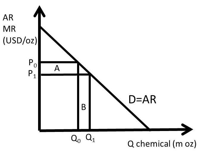
Figure 3.8 Per-Unit Revenues for a Monopolist: Agricultural Chemical
Increasing output by one unit from Q0 to Q1 has two effects on revenues: the monopolist gains area B, but loses area A. The monopolist can set price or quantity, but not both. If the output level is increased, consumers’ willingness to pay decreases, as the good becomes more available (less scarce). If quantity increases, price falls. The benefit of increasing output is equal to ΔQ*P1, since the firm sells one additional unit (ΔQ) at the price P1 (area B). The cost associated with increasing output by one unit is equal to ΔP*Q0, since the price decreases (ΔP) for all units sold (area A). The monopoly cannot increase quantity without causing the price to fall for all units sold. If the benefits outweigh the costs, the monopolist should increase output: if ΔQ*P1 > ΔP*Q0, increase output. Conversely, if increasing output lowers revenues (ΔQ*P1 < ΔP*Q0), then the firm should reduce output level.
3.3.2 The Relationship between MR and Ed
There is a useful relationship between marginal revenue (MR) and the price elasticity of demand (Ed). It is derived by taking the first derivative of the total revenue (TR) function. The product rule from calculus is used. The product rule states that the derivative of an equation with two functions is equal to the derivative of the first function times the second, plus the derivative of the second function times the first function, as in Equation 3.3.
(3.3) ∂(yz)/∂x = (∂y/∂x)z + (∂z/∂x)y
The product rule is used to find the derivative of the TR function. Price is a function of quantity for a firm with market power. Recall that MR = ∂TR/∂Q, and the equation for the elasticity of demand:
Ed = (∂Q/∂P)P/Q
This will be used in the derivation below.
TR = P(Q)Q
∂TR/∂Q = (∂P/∂Q)Q + (∂Q/∂Q)P
MR = (∂P/∂Q)Q + Pnext, divide and multiply by P:
MR = [(∂P/∂Q)Q/P]P + P
MR = [1/Ed]P + P
MR = P(1 + 1/Ed)
This is a useful equation for a monopoly, as it links the price elasticity of demand with the price that maximizes profits. The relationship can be seen in Figure 3.9.
(3.4) MR = P(1 + 1/Ed)
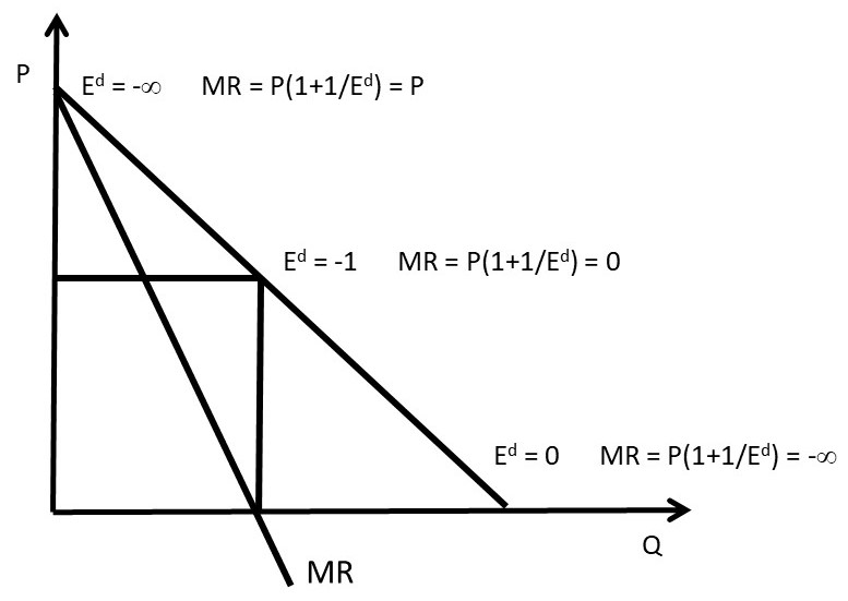
Figure 3.9 The Relationship between MR and Ed
At the vertical intercept, the elasticity of demand is equal to negative infinity (section 1.4.8). When this elasticity is substituted into the MR equation, the result is MR = P. The MR curve is equal to the demand curve at the vertical intercept. At the horizontal intercept, the price elasticity of demand is equal to zero (Section 1.4.8,, resulting in MR equal to negative infinity. If the MR curve were extended to the right, it would approach minus infinity as Q approached the horizontal intercept. At the midpoint of the demand curve, P is equal to Q, the price elasticity of demand is equal to -1, and MR = 0. The MR curve intersects the horizontal axis at the midpoint between the origin and the horizontal intercept.
This highlights the usefulness of knowing the elasticity of demand. The monopolist will want to be on the elastic portion of the demand curve, to the left of the midpoint, where marginal revenues are positive. The monopolist will avoid the inelastic portion of the demand curve by decreasing output until MR is positive. Intuitively, decreasing output makes the good more scarce, thereby increasing consumer willingness to pay for the good.
3.3.3 Pricing Rule I
The useful relationship between MR and Ed in Equation 3.4 can be used to derive a pricing rule.
MR = P(1 + 1/Ed)
MR = P + P/Ed
Assume profit maximization [MR = MC]
MC = P + P/Ed
–P/Ed = P – MC
–1/Ed = (P – MC)/P
(P – MC)/P = –1/Ed
This pricing rule relates the price markup over the cost of production (P – MC) to the price elasticity of demand.
(3.5) (P – MC)/P = –1/Ed
A competitive firm is a price taker, as shown in Figure 3.10. The market for a good is depicted on the left hand side of Figure 2.10, and the individual competitive firm is found on the right hand side. The market price is found at the market equilibrium (left panel), where market demand equals market supply. For the individual competitive firm, price is fixed and given at the market level (right panel). Therefore, the demand curve facing the competitive firm is perfectly horizontal (elastic), as shown in Figure 3.10.
The price is fixed and given, no matter what quantity the firm sells. The price elasticity of demand for a competitive firm is equal to negative infinity: Ed = -. When substituted into Equation 3.5, this yields (P – MC)P = 0, since dividing by infinity equals zero. This demonstrates that a competitive firm cannot increase price above the cost of production: P = MC. If a competitive firm increases price, it loses all customers: they have perfect substitutes available from numerous other firms.
Monopoly power, also called market power, is the ability to set price. Firms with market power face a downward sloping demand curve. Assume that a monopolist has a demand curve with the price elasticity of demand equal to negative two: Ed = -2. When this is substituted into Equation 3.5, the result is: (P – MC)/P = 0.5. Multiply both sides of this equation by price (P): (P – MC) = 0.5P, or 0.5P = MC, which yields: P = 2MC. The markup (the level of price above marginal cost) for this firm is two times the cost of production. The size of the optimal, profit-maximizing markup is dictated by the elasticity of demand. Firms with responsive consumers, or elastic demands, will not want to charge a large markup. Firms with inelastic demands are able to charge a higher markup, as their consumers are less responsive to price changes.

Figure 3.10 The Demand Curve of a Competitive Firm
In the next section, we will discuss several important features of a monopolist, including the absence of a supply curve, the effect of a tax on monopoly price, and a multiplant monopolist.
3.4 Monopoly Characteristics
3.4.1 The Absence of a Supply Curve for a Monopolist
There is no supply curve for a monopolist. This differs from a competitive industry, where there is a one-to-one correspondence between price (P) and quantity supplied (Qs). For a monopoly, the price depends on the shape of the demand curve, as shown in Figure 3.11. A mathematical “function” is defined as a one-to-one correspondence between each point in the range (x) and the domain (y). A supply curve, then, requires a single price (P) for each quantity (Q). This graph shows that there is more than one price associated with each quantity. At quantity Q0, for demand curve D1, the monopolist maximizes profits by setting MR1 = MC, which results in price P1. However, for demand curve D2, the monopolist would set MR2=MC, and charge a lower price, P2. Since there is more than one price associated with a single quantity (Q0), there is no one-to-one correspondence between price and quantity supplied, and no supply curve for a monopolist.
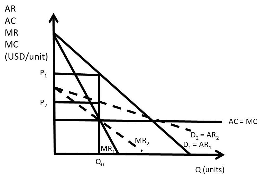
Figure 3.11 Absence of a Supply Curve for a Monopolist
3.4.2 The Effect of a Tax on a Monopolist’s Price
In a competitive industry, a tax results in an increase in price that is based on the incidence of the tax. The price increase is a fraction of the tax, less than the tax amount. The tax incidence depends on the magnitude of the elasticities of supply and demand. In a monopoly, it is possible that the price increase from a tax is greater than the tax itself, as shown in Figure 3.12. This is an interesting and nonintuitive result!
Before the tax, the monopolist sets MR = MC at Q0, and sets price at P0. After the tax is imposed, the marginal costs increase to C + t. The monopolist sets MR = MC = C + t, produces quantity Q1, and charges price P1. The increase in price (P1 – P0) is larger than the tax rate (t), the vertical distance between the C + t and MC lines. In this case, consumers of the monopoly good are paying more than 100 percent of the tax rate. This is because of the shape of the demand curve: it is profitable for the monopoly to reduce quantity produced to increase the price.
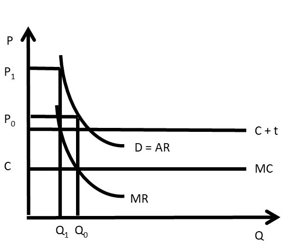
Figure 3.12 The Effect of a Tax on a Monopolist’s Price
3.4.3 Multiplant Monopolist
Suppose that a monopoly has two or more plants (factories). How does the monopolist determine how much output should be produced at each plant? Profit-maximization suggests two guidelines for the multiplant monopolist. Suppose that the monopolist operates n plants.
(1) Set MC equal across all plants: MC1 = MC2 = … =MCn, and
(2) Set MR = MC in all plants.
A mathematical model of a multiplant monopolist demonstrates profit-maximization. The result is interesting and important, as it shows that multiplant firms will not always close older, less efficient plants. This is true even if the older plants have higher production costs than newer, more efficient plants.
Suppose that a monopolist has two plants, and total output (QT) is the sum of output produced in plant 1 (Q1) and plant 2 (Q2).
(3.6) Q1 + Q2 = QT
The profit-maximizing model for the two-plant monopolist yields the solution. The costs of producing output in each plant differ. Assume that the old plant (plant 1) is less efficient than the new plant (plant 2): C1 > C2.
max π = TR – TC
= P(QT)QT – C1(Q1) – C2(Q2)
∂π/∂Q1 = ∂TR/∂Q1 – C1’(Q1) = 0
∂π/∂Q2 = ∂TR/∂Q2 – C2’(Q2) = 0
The profit-maximizing solution is:
(3.7) MR = MC1 = MC2
The multiplant monopolist solution is shown in Figure 3.13. The marginal cost curve for plant 1 is higher than the marginal cost curve for plant 2, reflecting the older, less efficient plant. Rather than shutting the less efficient plant down, the monopolist should produce some output in each plant, and set the MC of each plant equal to MR, as shown in the graph. Let MCT be the total (sum) of the marginal cost curves: MT = MC1 + MC2. The profit maximizing quantity (QT) is found by setting MR equal to MCT. At the profit maximizing quantity (QT), the monopolist sets price equal to P, found by plugging QT into the consumers’ willingness to pay, or the demand curve (D).
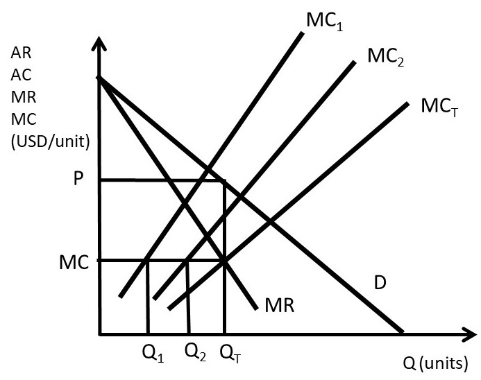
Figure 3.13 Multiplant Monopolist
To find the quantity to produce in each plant, the firm sets MC1 = MC2 = MCT to find the profit-maximizing level of output in each plant: Q1 and Q2. The outcome of the multiplant monopolist yields useful conclusions for any firm: continue using any input, plant, or resource until marginal costs equal marginal revenues. Less efficient resources can be usefully employed, even if more efficient resources are available. The next section will explore the determinants and measurement of monopoly power, also called market power.
3.5 Monopoly Power
In this section, the determinants and measurement of monopoly power are examined.
3.5.1 The Lerner Index of Monopoly Power
Economists use the Lerner Index to measure monopoly power, also called market power. The index is the percent markup of price over marginal cost.
(3.8) L = (P – MC)/P
The Lerner Index is a positive number (L ≥ 0), increasing in the amount of market power. A perfectly competitive firm has a Lerner Index equal to zero (L = 0), since price is equal to marginal cost (P = MC). A monopolist will have a Lerner Index greater than zero, and the index will be determined by the amount of market power that the firm has. A larger Lerner Index indicates more market power. In Section 3.3.3, a Pricing Rule was derived: (P – MC)/P = – 1/Ed, where Ed is the price elasticity of demand. Substitution of this pricing rule into the definition of the Lerner Index provides the relationship between the percent markup and the price elasticity of demand.
(3.9) L = (P – MC)/P = – 1/Ed
An example of a Lerner Index might be Big Macs. There are substitutes available for Big Macs, so if the price increases, consumers can buy a competing brand such as Whoppers. In the case of a good with close substitutes, the price elasticity of demand is larger (more elastic), causing the percent markup to be smaller: the Lerner Index is relatively small. A monopoly is defined as a single seller in an industry with no close substitutes. Therefore, a monopoly that produces a good with no close substitutes would have a higher Lerner Index.
A second pricing rule can be derived from equation (3.9), if we assume that the firm maximizes profits (MR = MC). In that case, the relationship between price and marginal revenue is equal to: MR = P(1 + 1/Ed). If profit-maximization (MR = MC) is assumed, then:
(3.10) MC = P(1 + 1/Ed)
Rearranging:
(3.11) P = MC/(1 + 1/Ed)
This is a useful equation, as it relates price to marginal cost. For example, a perfectly competitive firm has a perfectly elastic demand curve (Ed = negative infinity). Substitution of this elasticity into the pricing rule yields P = MC. For a monopoly that has a price elasticity equal to –2, P = 2MC. The price is two times the production costs in this case. To summarize:
(1) if Ed is large, the firm has less market power, and a small markup
(2) if Ed is small, the firm has more market power, and a large markup.
A monopoly example is useful to review monopoly and the Lerner Index. Suppose that the inverse demand curve facing a monopoly is given by: P = 500 – 10Q. The monopoly production costs are given by: C(Q) = 10Q2 + 100Q. Profit-maximization yields the optimal monopoly price and quantity.
max π = TR – TC
= P(Q)Q – C(Q)
= (500 – 10Q)Q – (10Q2 + 100Q)
= 500Q – 10Q2 – 10Q2 – 100Q
∂π/∂Q= 500 – 20Q – 20Q – 100 = 0
40Q = 400
Q* = 10 units
P* = 500 – 10Q* = 500 – 100 = 400 USD/unit.
To calculate the value of the Lerner Index, price and marginal cost are needed (equation 3.9).
MC = C’(Q) = 20Q + 100.
MC* = 20(10) + 100 = 300 units
L = (P – MC)/P = (400 – 300)/400 = 100/400 = 0.25
This result can be checked with the pricing rule: (P – MC)/P = – 1/Ed.
Ed = (∂Q/∂P)(P/Q)
For this monopoly, ∂P/∂Q = –10. This is the first derivative of the inverse demand function. Therefore, ∂Q/∂P = – 1/10.
Ed = (∂Q/∂P)(P/Q) = (– 1/10)(400/10) = – 400/100 = – 4.
L = (P – MC)/P = – 1/Ed = –1/–4 = 0.25.
The same result was achieved using both methods, so the Lerner Index for this monopoly is equal to 0.25.
3.5.2 Welfare Effects of Monopoly
The welfare effects of a market or policy change are summarized as, “who is helped, who is hurt, and by how much.” To measure the welfare impact of monopoly, the monopoly outcome is compared with perfect competition. In competition, the price is equal to marginal cost (P = MC), as in Figure 3.14. The competitive price and quantity are Pc and Qc. The monopoly price and quantity are found where marginal revenue equals marginal cost (MR = MC): PM and QM. The graph indicates that the monopoly reduces output from the competitive level in order to increase the price (PM > Pc and QM < Qc). The welfare analysis of a monopoly relative to competition is straightforward.
ΔCS = – AB
ΔPS = +A – C
ΔSW = – BC
DWL = BC
Consumers are losers, and the benefits of monopoly depend on the magnitudes of areas A and C. Since a monopolist faces an inelastic supply curve (no close substitutes), area A is likely to be larger than area C, making the net benefits of monopoly positive.
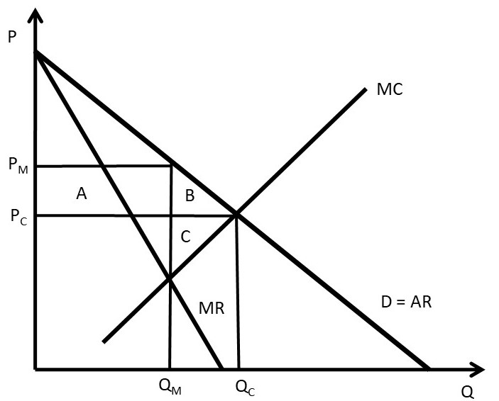
Figure 3.14 Welfare Effects of Monopoly
The monopoly example from the previous section 3.5.1 shows the magnitude of the welfare changes. From above, the inverse demand curve is given by P = 500 – 10Q, and the costs are given by C(Q) = 10Q2 + 100Q. In this case, PM = 400 USD/unit and QM = 10 units (see section 3.5.1 above). The competitive solution is found where the demand curve intersects the marginal cost curve.
500 – 10Q = 20Q + 100
30Q = 400
Qc = 13.3 units
Pc = 500 – 10(13.3) = 500 – 133 = 367 USD/unit
ΔCS = – AB = –(400 – 367)10 – (0.5)(400 – 367)(13.3 – 10) = – 330 –54.5 = – 384.5 USD
ΔPS = +A – C = +330 – (0.5)(367 – 300)(13.3 – 10) = +330 – 110.5 = +219.5 USD
ΔSW = – BC = (0.5)(100)(3.3) = – 165 USD
DWL = BC = 165 USD
The welfare analysis of monopoly has been used by the government to justify breaking up monopolies into smaller, competing firms. In food and agriculture, many individuals and groups are opposed to large agribusiness firms. One concern is that these large firms have monopoly power, which results in a transfer of welfare from consumers to producers, and deadweight loss to society. It will be shown below that outlawing or banning monopolies would have both benefits and costs. There is some economic justification for the existence of large firms due to economies of scale and natural monopoly, as will be explored below. Next, the sources of monopoly power will be listed and explained.
3.5.3 Sources of Monopoly Power
There are three major sources of monopoly power:
(1) the price elasticity of demand (Ed),
(2) the number of firms in a market, and
(3) interaction among firms.
The price elasticity of demand is the most important determinant of market power, due to the pricing rule: L = (P – MC)/P = – 1/Ed. When the price elasticity is large ( |Ed| > 1), demand is relatively elastic, and the firm has less market power. When the price elasticity is small ( |Ed| < 1), demand is relatively inelastic, and the firm has more market power.
The price elasticity of demand depends on how large the firm is relative to the market. The firm’s price elasticity of demand is always more elastic than the market demand:
|Edfirm| > |Edmarket| .
If the price of the firm’s output is increased, consumers can substitute into outputs produced by other firms. However, if all firms in the market increase the price of the good, consumers have no close substitutes, so must pay the higher price (Figure 3.15). Therefore, the firm’s price elasticity of demand is more elastic than the market demand. The firm’s price elasticity of demand depends on how large the firm is relative to the other firms in the market.
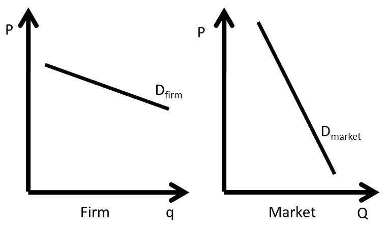
Figure 3.15 Price Elasticity of Demand for Firm and Industry
The second determinant of market power is the number of firms in an industry. This is related to Figure 3.15. If a firm is the only seller in an industry, then the firm is the same as the market, and the price elasticity of demand is the same for both the firm and the market. The more firms there are in a market, the more substitutes a consumer has available, making the price elasticity of demand more elastic as the number of firms increases. In the extreme case, a perfectly competitive firm has numerous other firms in the industry, causing the demand curve to be perfectly elastic, P = MC, and L = 0. To summarize, the more firms there are in an industry, the less market power the firm has.
The number of firms in an industry is determined by the ease or difficulty of entry. This market feature is captured by the concept of, “Barriers to Entry.” Barriers to entry include:
(1) patents,
(2) copyrights,
(3) contracts,
(4) economies to scale (natural monopoly),
(5) excess capacity, and
(6) licenses.
Each of these barriers to entry increases the difficulty of entering a market when positive economic profits exist. Economies to scale and natural monopoly are defined and described in the next section. The number of firms is important, but the number of “major firms” is also important. Some industries are characterized by one or two dominant firms. These large firms often exert market power.
The third source of market power is interaction among firms. This will be extensively discussed in Chapter 5, “Oligopoly.” If firms compete aggressively with each other, less market power results. On the other hand, if firms cooperate and act together, the firms can have more market power. When firms join together, they are said to “collude,” or act as if they were a single firm. These strategic interactions between firms form the heart of the discussion in Chapter 5, and the foundation for game theory, explored in Chapters 6 and 7.
3.5.4 Natural Monopoly
A natural monopoly is a firm that has a high level of costs that do not vary with output.
Natural Monopoly = A firm characterized by large fixed costs.
Recall that total costs are the sum of total variable costs and total fixed costs (TC = TVC + TFC). The fixed costs are those costs that do not vary with the level of output. When fixed costs are high, then average total costs are declining, as seen in Figure 3.16.
Another way of describing high fixed costs is the term, “economies of scale.”
Economies of Scale = Per-unit costs of production decrease when output is increased.
Figure 3.16 shows the defining characteristic of a natural monopoly: declining average costs (AC). This means that the demand curve intersects the AC curve while it is declining. At some point, the average costs will increase, but for firms characterized by economies of scale, the relevant range of the AC curve is the declining portion, of the left side of a typical “U-shaped” cost function.
The reason for the name, “natural monopoly” can also be found in Figure 3.16. The demand curve has a portion above the AC curve, so positive profits are possible. Suppose that the monopoly was making positive economic profits, and attracted a competitor into the industry. The second firm would cause the demand facing each of the two firms to be cut in half. This possibility can be seen in Figure 3.16: if two firms served the customers, each firm would have a demand curve equal to the MR curve. This is because for a linear demand curve, the MR curve has the same y-intercept and twice the slope. Notice the position of the MR curve for a natural monopoly: it lies everywhere below the AC curve. Therefore, positive profits are not possible for two firms serving this market. The demand is not large enough to cover the fixed costs.
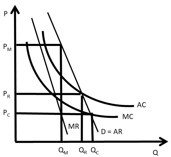
Fig 3.16 Natural Monopoly
The fixed costs are typically large investments that must be made before the good can be sold. For example, an electricity company must build both a huge generating plant and a distribution network that connects all residences and businesses to the power grid. These enormous costs do not vary with the level of output: they must be paid whether the firm sells zero kilowatt hours or one million kilowatt hours. The average fixed costs decline as they are spread out over larger quantities (AFC = TFC/Q). As the output (Q) increases, average costs (AC = TC/Q) decline.
This feature is true for many large businesses, and provides economic justification for large firms: the per-unit costs of production are smaller, providing lower costs to consumers. There is a tradeoff for consumers who purchase goods from large firms: the cost is lower due to economies of scale, but the firm may have market power, which can result in higher prices. This tradeoff makes the economic analysis of large firms both fascinating and important to society. Current examples include the giant technology companies Microsoft, Apple, Google, and Amazon.
Natural monopolies have important implications for how large businesses provide goods to consumers, as is explicitly shown in Figure 3.16. The industry in Figure 3.16 is a natural monopoly, since demand intersects average costs while they are declining. If a single firm was in the depicted industry, it would set marginal costs equal to marginal revenues (MR = MC), and produce and sell QM units of output at a price equal to PM. The price is high: consumers lose welfare and society is faced with deadweight losses.
If competition were possible, price would be set at marginal cost (P = MC). The resulting price and quantity under competition would be PC and QC (Figure 3.16. This is a desirable outcome for the consumers. However, there is a major problem with this outcome: price is below average costs, and any business firm that charged the competitive price PC would be forced out of business. In this case, the firm does not have enough revenue to cover the fixed costs. The natural monopoly is considered a “market failure” since there is no good market-based solution. A single monopoly firm could earn enough revenue to stay in business, but consumers would pay a high monopoly price PM). If competition occurred, the consumers would pay the cost of production (PC), but the firms would not cover their costs.
One solution to a natural monopoly is government regulation. If the government intervened, it could set the regulated price equal to average costs (PR = AC), and the regulated quantity equal to QR. This solves the problem of natural monopoly with a compromise: consumers pay a price just high enough to cover the firm’s average costs. This analysis explains why the government regulates many public utilities for electricity, natural gas, water, sewer, and garbage collection.
The next section will investigate monopsony, or a single buyer with market power.
3.6 Monopsony
A monopsony is defined as a market characterized by a single buyer.
Monopsony = single buyer of a good.
Monopsony power is market power of buyers. A firm with monopsony power is a buyer that is large enough relative to the market to influence the price of a good. Competitive firms are price takers: prices are fixed and given, no matter how little or how much they buy. In food and agriculture, beef packers are often accused of having market power, and pay lower prices for cattle than the competitive price. This section will explore the causes and consequences of monopsony power.
3.6.1 Terminology of Monopsony
Consider any decision from an economic point of view. Thinking like an economist results in comparing the benefits and costs of any decision. This section will apply economic thinking to the quantity and price of a purchase. It will follow the same economic approach that has been emphasized, but will define new terminology to distinguish the buyer’s decision (monopsony) from the seller’s decision (monopoly). It is useful to recall the meaning of supply and demand curves. The demand curve represents the consumers’ willingness and ability to pay for a good. The demand curve is downward sloping, reflecting scarcity: larger quantities are less scarce, and thus less valuable. The supply curve represents the producers’ cost of production, and is upward sloping. As more of a good is produced, the marginal costs of production increase, since it requires more resources to produce larger quantities. These economic principles will be useful in what follows, an analysis of a buyer’s decision to purchase a good.
The economic approach to the purchase of a good is to employ marginal decision making by continuing to purchase a good as long as the marginal benefits outweigh the marginal costs. The following terms are defined to aid in our analysis of buyer’s market power.
Marginal Value (MV) = The additional benefits of buying one more unit of a good.
Marginal Expenditure (ME) = The additional costs of buying one more unit of a good.
Average Expenditure (AE) = The price paid per unit of a good.
A review of competitive buyers and sellers is a good starting point for our analysis.
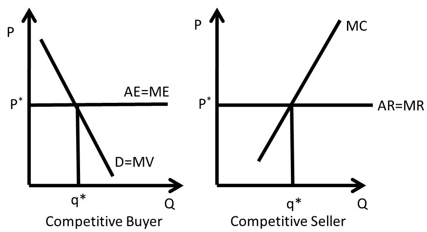
Figure 3.17 Competitive Buyer and Seller
Figure 3.17 demonstrates the competitive solution for a competitive buyer and a competitive seller. The competitive buyer faces a price that is fixed and given (P*). The price is constant because the buyer is so small relative to the market that her purchases do not affect the price. Average expenditures (AE) and marginal expenditures (ME) for this buyer are constant and equal (AE = ME). The buyer will continue purchasing the good until the marginal benefits, defined to be the marginal value (MV) are equal to marginal expenditures (ME) at q*, the optimal, profit-maximizing level of good to purchase.
A competitive seller takes the price as fixed and given (P*). The price is constant because the seller is so small relative to the market that his sales do not affect the price. Average revenues (AR) and marginal revenues (MR) for this seller are constant and equal (AR = MR). The seller will continue producing and selling the good until the marginal benefits, defined to be the marginal revenues (MR) are equal to marginal costs (MC) at q*, the optimal, profit-maximizing level of good to produce.
A monopsony uses the same decision making framework, comparing marginal benefits and marginal costs. The distinction is that a monopsony is large enough relative to the market to influence the price. Thus, the monopsony faces an upward-sloping supply curve: as the monopsony purchases more of the good, it drives the price up (Figure 3.18).
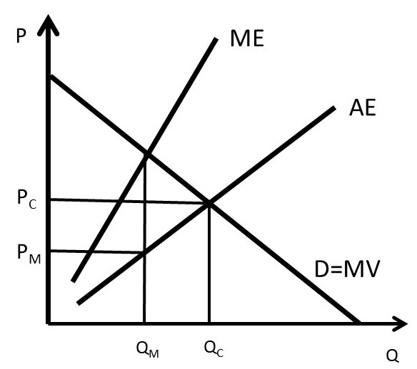
Figure 3.18 Monopsony
Since the firm is large, when it purchases more of a good, it drives the price higher. The average expenditure (AE) curve is the supply curve of the good faced by a monopsony. An example might be Ford Motor Company. When Ford purchases more steel (or glass or tires), the firm is so large relative to the market for steel that it drives the price up. Steel companies will need to buy more resources to produce more steel, and it will cost them more, since Ford is so large a buyer in the steel market.
The profit-maximizing solution is found by setting MV = ME, and purchasing the corresponding quantity QM. Note that the monopsony is restricting quantity, as a monopoly restricts output to drive the price up. However, a monopsony restricts quantity in order to drive the price down to PM. The monopsony is buying less than the competitive output (QC) and paying a price PM) lower than the competitive price (PM < PC).
It is worth answering the question, “why is ME > AE?” The monopsony faces an upward-sloping supply curve (AE). This reflects the higher cost of bringing more resources into the production of the good purchased by the monopsony. This can be seen in Figure 3.19. Next, the relationship between AE and ME is derived. This derivation will be familiar, as it is the same as the relationship between AR and MR from section 3.3.2 above. The derivation of ME uses the product rule.
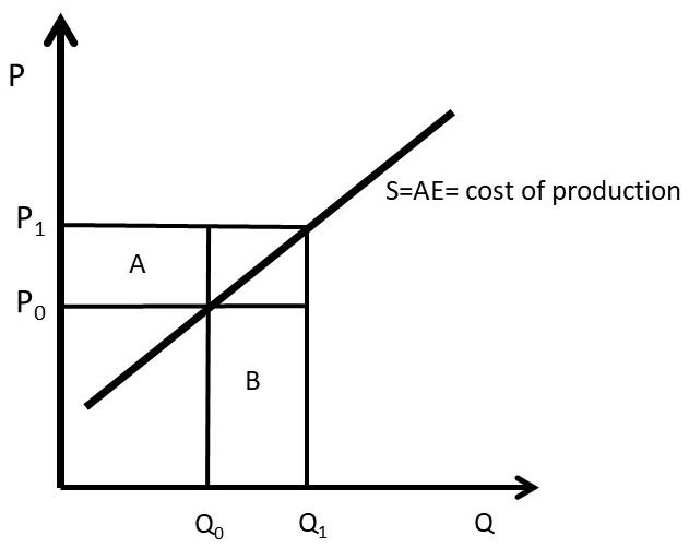
Figure 3.19 Monopsony Supply Curve
AE = P(Q)
TE = P(Q)Q
ME = ∂TE/∂Q = (∂P/∂Q)Q + P
ME = AE + (∂P/∂Q)Q
The first term in the expression for ME is AE, which corresponds to area B in Figure 3.19 (P0ΔQ). Average expenditure is equal to P0 at quantity Q0. The second term, (∂P/∂Q)Q, is equal to area A in the diagram. This area represents the change in price given a small change in quantity (∂P/∂Q), multiplied by the quantity (Q). For a competitive firm, (∂P/∂Q) = 0, since the competitive firm is a price taker. For a competitive firm, AE = ME, as shown in the left of Figure 3.17. For a monopsony, the firm pays the initial price plus the increase in price caused by an increase in output. The monopsony must pay this new price (P1 in Figure 3.19) for all units purchased (Q). This causes ME to be above AE.
It is instructive to view the monopoly graph next to the monopsony graph (Figure 3.20).
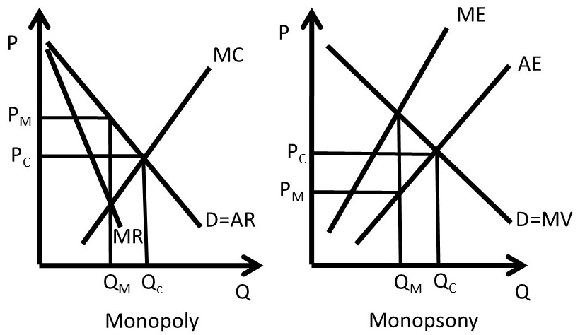
Figure 3.20 Monopoly and Monopsony
The monopoly in the left panel of Figure 3.20 restricts output to drive up the price. The monopoly output is less than the competitive output (QM < QC), and the monopoly price is higher than the competitive price (PM > PC). The monopsony in the right panel of Figure 3.20 restricts output to drive down the price (PM < PC). Both firms are maximizing profit by using the market characteristics that they face.
3.6.2 Welfare Effects of Monopsony
To measure the welfare impact of monopsony, the monopsony outcome is compared with perfect competition. In competition, the price is equal to marginal cost (PC = MC), as in Figure 3.21. The competitive price and quantity are Pc and Qc. The monopsony price and quantity are found where marginal value (MV) equals marginal expenditure (MV = ME): PM and QM. The graph indicates that the monopsony reduces output from the competitive level in order to decrease the price (PM < Pc and QM < Qc). The welfare analysis of a monopsony relative to competition is straightforward.
ΔCS = +A – B
ΔPS = –AC
ΔSW = – BC
DWL = BC
Consumers are winners, and the benefits of monopsony depend on the magnitudes of areas A and B.
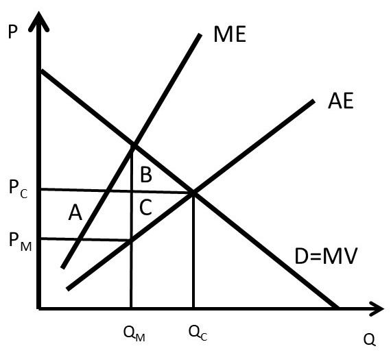
Figure 3.21 Welfare Effects of Monopsony
3.6.3 Sources of Monopsony Power
There are three major sources of monopsony power, analogous to the three determinants of monopoly power:
(1) the price elasticity of market supply (Es),
(2) the number of buyers in a market, and
(3) interaction among buyers.
The price elasticity of supply is the most important determinant of monopsony power, and the monopsony benefits from an inelastic supply curve. When the price elasticity is large (Es > 1), the supply is relatively elastic, and the firm has less market power. When the price elasticity is small (Es < 1), the demand is relatively inelastic, and the firm has more market power. This is shown in Figure 3.22.
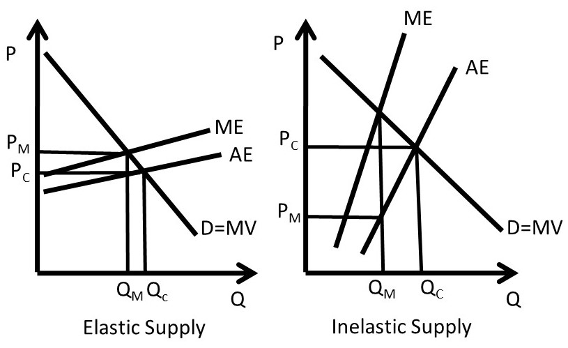
Figure 3.22 Price Elasticity of Supply Impact on Monopsony
The second determinant of monopsony power is the number of firms in an industry. If a firm is the only buyer in an industry, the firm is a monopsony, and has market power. The more firms there are in a market, the more competition the firm faces, and the less market power.
The third source of monopsony power is interaction among firms. If firms compete aggressively with each other, less monopsony power results. On the other hand, if firms cooperate and act together, the firms can have more monopsony power. The next Chapter will explore how firms with market power determine optimal prices.
