Main Body
Chapter 4. Pricing with Market Power
4.1 Introduction to Pricing with Market Power
In economics, the firm’s objective is assumed to be to maximize profits. Firms with market power do this by capturing consumer surplus, and converting it to producer surplus. In Figure 4.1, a monopoly finds the profit-maximizing price and quantity by setting MR equal to MC. This strategy maximizes profits for a firm setting a single price (PM) and charging all customers the same price. In some situations, it is possible for a monopolist to increase profits beyond the single price monopoly solution. Figure 4.1 shows that there are two sources of consumer willingness to pay that the monopoly has not taken advantage of by producing a quantity of QM and selling it at price PM.
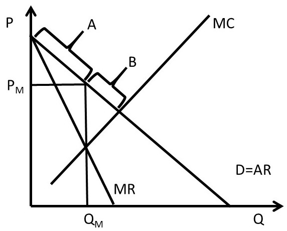
Figure 4.1 Pricing Strategy for Firms with Market Power
Area A along the demand curve represents consumers with a higher willingness to pay than the monopoly price PM. Area B represents consumers who have been priced out of the market, since the monopoly price is higher than their willingness to pay. These two groups of consumers represent two areas of untapped consumer surplus for a monopoly.
The monopoly price PM represents the profit-maximizing price if the monopolist is constrained to set only a single price, and charge all customers the same single price. However, if the monopolist could charge more than one price, it may be able to capture more consumer surplus (willingness to pay) and convert it into producer surplus (profits). This Chapter describes and explains several pricing strategies for firms with market power. These strategies enhance profits over and above the single price profit level shown in Figure 4.1. The strategies include price discrimination, peak-load pricing, and two-part pricing.
4.2 Price Discrimination
Price discrimination is the practice of charging different prices to different customers. There are three forms of price discrimination, defined and explained in what follows.
Price Discrimination = charging different prices to different customers.
4.2.1 First Degree Price Discrimination
First degree price discrimination is the extreme form of charging different prices to different consumers, and makes use of the concept of “reservation price.” A consumer’s maximum willingness to pay is defined to be their reservation price.
Reservation Price = The maximum price that a consumer is willing to pay for a good.
First Degree Price Discrimination = Charging each consumer her reservation price.
First degree price discrimination is shown in Figure 4.2, where the initial levels of consumer surplus (CS0) and producer surplus (PS0) are defined for the competitive equilibrium. The competitive quantity is QC, and the competitive price is PC. A monopoly could charge a price PM at quantity QM to maximize profits with a single price.
Each individual’s willingness to pay is given by a point on the demand curve. If the firm knows each consumer’s maximum willingness to pay, or reservation price, it can transfer all consumer surplus to producer surplus. The firm extracts every dollar of surplus available in the market by charging each consumer the maximum price that they are willing to pay. First degree price discrimination results in levels of producer surplus and consumer surplus PS1 and CS1, as shown in equation 4.1.
(4.1) PS1 = PS0 + CS0; CS1 = 0.
Every dollar of consumer surplus has been transferred to the firm. First degree price discrimination is also called, “Perfect Price Discrimination.”
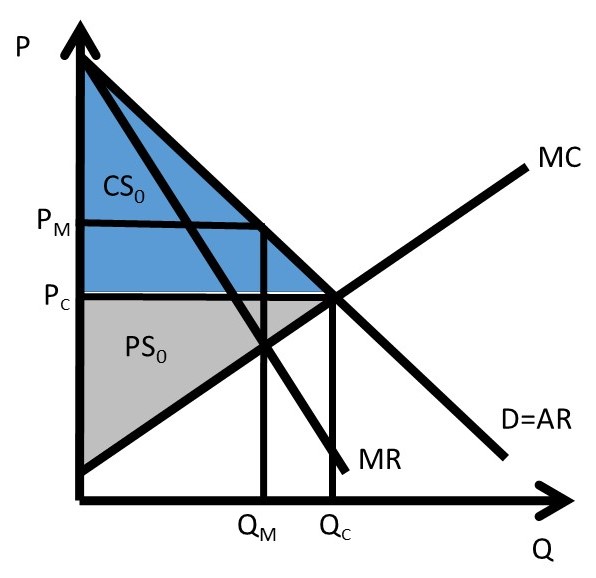
Figure 4.2 First Degree Price Discrimination
In most circumstances, it is difficult for the firm to practice first degree price discrimination. First, it is difficult to charge different prices to different consumers. In many cases, it is illegal to charge different prices to different people. Second, it is difficult and costly to elicit reservation prices from every consumer. Therefore, first degree price discrimination is an extreme, idealized case of charging different prices to different consumers. It is rare in the real world.
“Imperfect Price Discrimination” is a term used to describe markets that approach perfect price discrimination. Examples of imperfect price discrimination include car sales and college tuition rates for students in college. Car dealerships often post a “sticker price” and then lower the actual price, depending on how much the consumer is willing to pay. Successful car sales people are often those who have exceptional abilities to discern exactly how much each consumer is willing to pay, or their reservation price. Colleges and universities use imperfect price discrimination by offering scholarships and financial aid packages to students based on their willingness to enroll and attend an institution.
Imperfect price discrimination is shown in Figure 4.3, where different groups of consumers are charged different prices based on their willingness to pay. Price P1 is a high price to capture consumers with high willingness to pay, price P2 is the monopoly price (PM), and price P3 is the competitive price. If a firm can distinguish different consumer groups’ willingness to pay, it can enhance profits through this form of price discrimination.
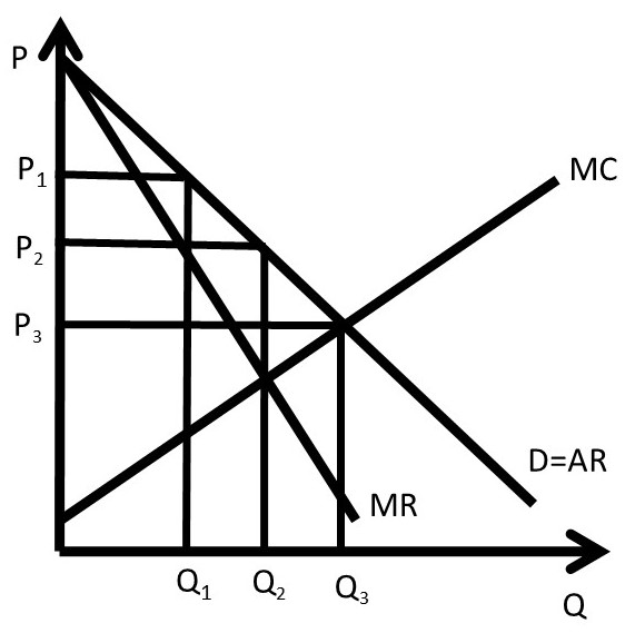
Figure 4.3 Imperfect Price Discrimination
4.2.2 Second Degree Price Discrimination
Second Degree Price Discrimination is a quantity discount.
Second Degree Price Discrimination = Charging different per-unit prices for different quantities of the same good.
Second degree price discrimination is a common form of pricing and packaging. Consider an example of two different sized packages of salsa with different prices per unit. Suppose that consumers have different preferences for different sized salsa packages, and different demand curves reflect this.
For simplicity, assume that there are two consumers (consumer 1 and consumer 2) and two choices of package size (A and B).
A: 8 oz jar, price = 2 USD, price per unit = 0.25 USD/oz
B: 32 oz jar, price = 4.80 USD, price per unit = 0.15 USD/oz
Figure 4.4 shows consumer demand for each of the two consumers.
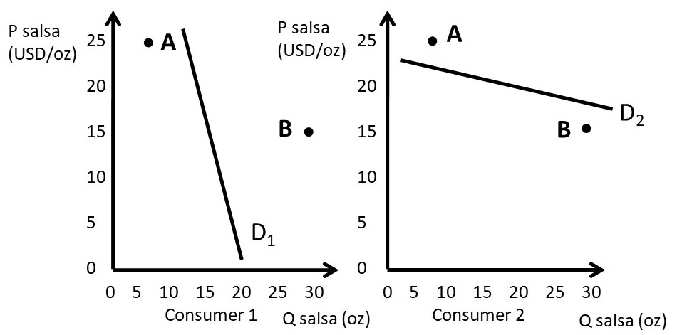
Figure 4.4 Second Degree Price Discrimination
Consumer 1 has a preference for smaller quantities. This consumer could be a single person who desires to purchase a small jar of salsa. Consumer 1’s demand curve demonstrates that she is willing to pay for the 8 ounce jar of salsa (A), but not the 32 ounce jar (B). This is because A lies below demand curve D1, but not B. On the other hand, consumer 2 desires the large jar of salsa, perhaps this is a family of four persons. Consumer 2 is willing to purchase the 32 ounce jar (B), but not the 8 ounce jar (A). This is because B lies below the demand curve D2, but not A.
It can be shown that the salsa firm can enhance profits by offering both sizes A and B. Assume that the costs of producing salsa are equal to ten cents per ounce:
MC = 0.10 USD/oz.
Situation One. Firm sells 8-ounce jar only.
Consumer 1 buys, Consumer 2 does not buy.
Q = 8 oz; P = 0.25 USD/oz; MC = 0.10 USD/oz
π1 = (P – MC)Q = (0.25 – 0.10)8 = (0.15)8 = 1.20 USD
Situation Two. Firm sells 32-ounce jar only.
Consumer 2 buys, Consumer 1 does not buy.
Q = 32 oz; P = 0.15 USD/oz; MC = 0.10 USD/oz
π2 = (P – MC)Q = (0.15 – 0.10)32 = (0.05)32 = 1.60 USD
Situation Three. Firm sells both 8-ounce and 32-ounce jars.
Consumer 1 buys 8 ounce jar, Consumer 2 buys 32 ounce jar.
π3 = (0.25 – 0.10)8 + (0.15 – 0.10)32 = (0.15)8 + (0.05)32 = 2.80 USD
Profits are larger if different sized packages are sold at the same time. Second degree price discrimination takes advantage of differences between consumers, and is usually more profitable than offering a good in only one package size. This explains the huge diversity of package sizes available for a large number of consumer goods.
4.2.3 Third Degree Price Discrimination
Third degree price discrimination is a practice of charging different prices to different consumer groups.
Third Degree Price Discrimination = Charging different prices to different consumer groups.
A firm that faces more than one group of consumers can increase profits by offering a good at different prices to groups of consumers with different levels of willingness to pay. The firm will maximize profits by setting the marginal revenue (MR) for each consumer group equal to the marginal cost of production (MC). This solution is shown in equation 4.2 for two consumer groups:
(4.2) MR1 = MR2 = MC.
Two things are interesting about this result. First, the firm practicing third degree price discrimination is simply following the profit-maximizing strategy of continuing any activity as long as the benefits outweigh the costs. The firm will stop when marginal benefits from selling the good to both groups are equal to the marginal costs of producing the good. Second, this solution is similar to the solution for the multiplant monopoly: MC1 = MC2 = MR. Profit-maximizing firms use the same strategy for multiple plants and multiple consumers groups: set MR equal to MC in all circumstances.
Movie theaters often offer a student discount to students, as well as discounts for children, senior citizens, and military personnel. It may seem as if the theaters and other firms that offer these discounts are being nice to these groups. In reality, however, the firms are practicing third degree price discrimination to maximize profits! These groups of consumers have more elastic demands for movies, and would purchase a smaller number of movie tickets if the price was not discounted for them. A numerical example will demonstrate how third degree price discrimination works. Suppose that movie tickets are in thousands.
Movie ticket price = 12 USD/ticket
Student ticket price = 7 USD/ticket
Inverse Demand for movies: P1 = 20 – 4Q1
Inverse Demand for students: P2 = 10 – Q2
MC = 4 USD/ticket
max π = TR – TC
= TR1 – TC1 + TR2 – TC2
= P1Q1 – 4Q1 + P2Q2 – 4Q2
= (20 – 4Q1)Q1 – 4Q1 + (10 – Q2)Q2 – 4Q2
= 20Q1 – 4Q12 – 4Q1 + 10Q2 – Q22 – 4Q2
∂π/∂Q1 = 20 – 8Q1 – 4 = 0
8Q1 = 16
Q1* = 2 thousand movie tickets
P1* = 20 – 4(2) = 12 USD/ticket
∂π/∂Q2 = 10 – 2Q2 – 4 = 0
2Q2 = 6
Q2* = 3 thousand student movie tickets
P2* = 10 – (3) = 7 USD/ticket for students
The third degree price discrimination strategy is graphed in Figure 4.5.
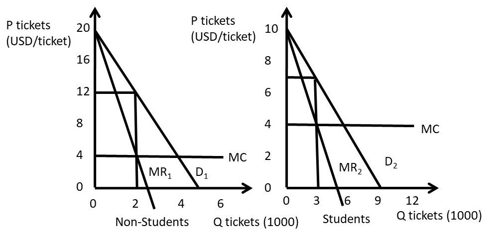
Figure 4.5 Third Degree Price Discrimination
A pricing rule for third degree price discrimination can be derived. Recall the pricing rule that was derived for a monopoly in Chapter 3:
(4.3) MR = P[1 + (1/Ed)]
This pricing rule can be extended to include two groups of consumers, as follows.
MR1 = MR2 = MC
P1[1 + (1/E1)] = P2[1 + (1/E2)]
P1/P2 = [1 + (1/E2)] / [1 + (1/E1)]
The pricing rule for the third degree price discriminating firm shows that the highest price is charged to the consumer group with the smallest (most inelastic) price elasticity of demand (Ed). This follows what we have learned about the elasticity of demand: consumers with an elastic demand will switch to a substitute good if the price increases, whereas consumers with an inelastic demand are more likely to pay the price increase.
The next section will present intertemporal price discrimination, or charging different prices at different times.
4.3 Intertemporal Price Discrimination
Intertemporal price discrimination provides a method for firms to separate consumer groups based on willingness to pay. The strategy involves charging a high price initially, then lowering price after time passes. Many technology products and recently-released products follow this strategy.
Intertemporal Price Discrimination = charging a high price initially, then lowering price after time passes.
Intertemporal price discrimination is similar to second degree price discrimination, but charges a different price across time. Second degree price discrimination charges a different price for different quantities at the same time. Intertemporal price discrimination is shown in Figure 4.6.
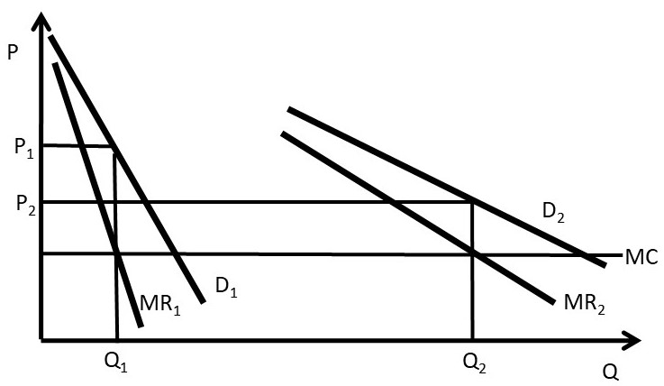
Figure 4.6 Intertemporal Price Discrimination, Graph One
The first group has a higher willingness to pay for the good, as shown by demand curve D1. This group will pay the higher initial price charged by the firm. A new iPhone release is a good example. Over time, Apple will lower the price to capture additional consumer groups, such as group two in Figure 4.6. In this fashion, the firm will extract a larger amount of consumer surplus than with a single price.
Intertemporal price discrimination can also be shown in a slightly different graph. The key feature of intertemporal price discrimination is a high initial price, followed by lower prices charged over time, as shown in Figure 4.7. In this graph, the firm initially charges price Pt to capture the high willingness to pay of some consumers. Over time, the firm lowers price to Pt+1, and later to Pt+2 to capture consumer groups with lower willingness to pay.
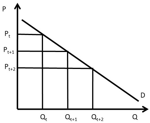
Figure 4.7 Intertemporal Price Discrimination, Graph Two
The concept of intertemporal price discrimination explains why new products are often priced at high prices, and the price is lowered over time. In the next section, peak-load pricing will be introduced.
4.4 Peak Load Pricing
The demand for many goods is larger during certain times of the day or week. For example, roads are congested during rush hours during the morning and evening commutes. Electricity has larger demand during the day than at night. Ski resorts have large (peak) demands during the weekends, and smaller demand during the week.
Peak Load Pricing = Charging a high price during demand peaks, and a lower price during off-peak time periods.
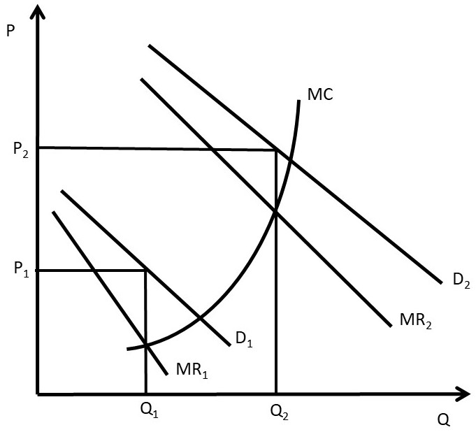
Figure 4.8 Peak Load Pricing
Figure 4.8 demonstrates the demand for electricity during the day. Demand curve D1 represents demand at off-peak hours at night. The electricity utility company will charge a price P1 for the off-peak hours. The costs of producing electricity increase dramatically during peak hours. Electricity generation reaches the capacity of the generating plants, causing larger quantities of electricity to be expensive to produce. For large coal-fired plants, when capacity is reached, the firm will use natural gas to generate the peak demand. To cover these higher costs, the firm will charge the higher price P2 during peak hours. The same graph represents a large number of other goods that have peak demand at different times during a day, week, or year (ski resorts, toll roads, parking lots, etc.).
Economic efficiency is greatly improved by charging higher prices during peak times. If the utility were required to charge a single price at all times, it would lose the ability to charge consumers an appropriate price during peak demand periods. Charging a higher price during peak hours provides an incentive for consumers to switch consumption to off-peak hours. This saves society resources, since costs are lower during those times.
An example is electricity consumption. If consumers are charged higher prices during peak hours, they are able to shift some electricity demand to night, the off-peak hours. Dishwashers, laundry, and bathing can be shifted to off-peak hours, saving the consumer money and saving society resources. Electricity companies also promote “smart grid” technology that automatically turns thermostats down when individuals and families are not at home… saving the consumer and society money.
The next section will discuss a two-part tariff, or charging consumers a fixed fee for the right to purchase a good, and a per-unit fee for each unit purchased.
4.5 Two-Part Pricing
A monopoly or any firm with market power can increase profits by charging a price structure with a fixed component, or entry fee, and a variable component, or usage fee.
Two-Part Pricing (also called Two Part Tariff) = A form of pricing in which consumers are charged both an entry fee (fixed price) and a usage fee (per-unit price).
Examples of two-part pricing include a phone contract that charges a fixed monthly charge and a per-minute charge for use of the phone. Amusement parks often charge an admission fee and an additional price per ride. Golf clubs typically charge an initiation fee and then usage fees based on meals eaten and golf rounds played. College football tickets usually require a “donation” to the athletic department, used for scholarships, and a per-ticket charge for the tickets.
Two-part pricing is shown in Figure 4.9, where a monopoly graph is presented.
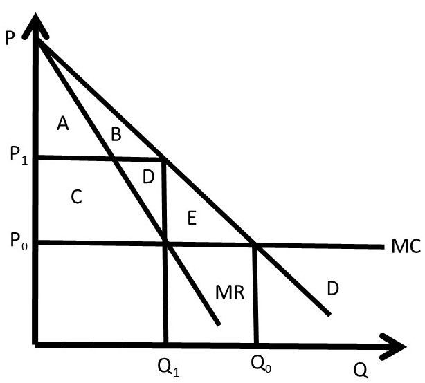
Figure 4.9 Two-Part Pricing
Suppose that the graph represents an individual consumer’s demand. In competitive equilibrium (subscript 0), price is equal to MC, output is equal to Q0, and producer and consumer surplus are given by:
PS0 = 0
CS0 = +ABCDE
The firm charges a price equal to the constant marginal cost (P = MC), and there is no producer surplus. Consumers receive the total area between the demand curve (willingness to pay) and the price line (price paid), equal to area ABCDE.
A profit-maximizing firm (subscript 1) that charged a single price would maximize profits by producing Q1 units of the good, and charging a price of P1. Surplus levels would be:
PS1 = +CD
CS1 = +AB
In this case, consumers have transferred areas C and D to producers, but still have surplus equal to area AB. Producers interested in increasing profits could devise a two-part pricing strategy that transfers more consumer surplus into producer surplus. Since CS > 0, consumers are willing to pay more than the monopoly price, and firms can extract a greater level of consumer surplus. The firm could charge an entry fee (T), and consumers would be willing to pay as long as the fee was less than their consumer surplus at the monopoly level (CS1 = AB).
Consider the following two-part pricing scheme (subscript 2):
Usage fee: P2 = MC
Entry fee: T = A+B+C+D+E [T is set equal CS0 = CS under competition]
PS2 = +ABCDE
CS2 = 0
With a two-part pricing scheme, the firm has extracted every dollar of willingness to pay from consumers. The total amount of producer surplus under two-part pricing is given by:
PS2 = T + (P2 – MC)Q2 = ABCDE
Notice that the firm earns zero profit from the usage fee (P2 = per-unit fee), since it sets the usage fee equal to the cost of production (P2 = MC). All of the profits come from the entry fee (T = fixed price) in this case.
To summarize, a two-part tariff for consumers with identical demands would (1) set usage fee (price per unit) equal to MC (P = MC), and (2) set a membership fee (entry fee) equal to consumer surplus at this price (T = CS at P = MC). The two-part price will result in (1) CS = 0, and (2) PS = T + (P – MC)Q = T.
A numerical example will further elucidate the two-part price. Assume that an individual’s inverse demand curve is given by: P = 20 – 2Q, and the cost function is C(Q) = 2Q. The firm seeks to find the optimal, profit-maximizing two-part tariff. The situation is shown in Figure 4.10.
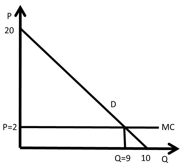
Figure 4.10 Two-Part Pricing Example
The firm will set the usage fee (per-unit price) equal to marginal cost: P* = MC = 2. At this price, the quantity sold is found by substitution of the price into the inverse demand function: 2 = 20 – 2Q, or 2Q = 18, Q* = 9 units, as shown in Figure 4.10. Next, the firm will determine the entry fee (fixed price), by calculating the area of consumer surplus at this price: CS = 0.5(20 – 2)(9 – 0) = 0.5(18)(9) = 9*9 = 81 USD. Therefore, the firm sets the usage fee: T = 81 USD. The resulting levels of surplus are CS = 0 and PS = 81 USD. To summarize, the optimal two-part tariff is to set the usage fee equal to marginal cost and the entry fee equal to the level of consumer surplus at that price: P* = 2 USD/unit, T* = 81 USD.
In our investigation of two-part pricing, identical consumer demands have been assumed. In the real world, consumer demands may differ quite markedly across individuals. Given this possibility, the two-part pricing strategy can be summarized as follows.
(1) If consumer demands are nearly identical, a two-part pricing scheme could increase profits by charging a price close to marginal cost and an entry fee.
(2) If consumer demands are different, a two-part pricing scheme or a single price scheme could be utilized by setting a price well above marginal cost and a lower entry fee to capture all consumers. Or, set a single price.
In the next section, commodity bundling will be explained and explored.
4.6 Bundling
The practice of bundling is that of selling two or more goods together as a package.
Bundling = The practice of selling two or more goods together as a package.
Bundling is a widely-practiced sales strategy that takes advantage of differences in consumer willingness to pay for different goods. McDonalds Happy Meals are an example of bundling, since the customer purchases a hamburger, French fries, beverage, and toy as a single purchase. McDonalds was an innovator in bundling, and has expanded the practice to include “Value Meals.” Communication companies often package internet service, cable television, and phone service together into a package.
4.6.1 Bundling Examples
A simple example of bundling is a value meal at a fast food restaurant. To make things simple, assume that there are two consumers (A and B), two products (burger and fries) and marginal costs are equal to zero. The zero-cost assumption is not realistic, but the model results do not change when we assume zero costs.
Table 4.1 shows the reservation prices (willingness to pay) for both consumers for each good.
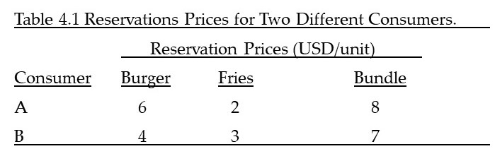
Recall that the reservation price is the maximum amount that a consumer is willing to pay for a good. The reservation price for the bundle (shown in the right column of table 4.1) is simply the sum of the two reservation prices for the burger and fries. Next, a comparison is made between selling the two good individually versus selling them as a bundle.
CASE ONE: Sell each product individually.
Πburger 1. If set Pburger = 6 USD/unit, A buys, Πburger = 6*1 = 6 USD
2. If set Pburger = 4 USD/unit, A and B buy, Πburger = 4*2 = 8 USD
>>>Set P*burger = 4 USD/unit; Πburger = 8 USD
Πfries 1. If set Pfries = 2 USD/unit, A and B buy, Πfries = 2*2 = 4 USD
2. If set Pfries = 3 USD/unit, B buys, Πfries = 3*1 = 3 USD
>>>Set P*fries = 2 USD/unit; Πfries = 4 USD
Πtotal individualΠtotal individual = PbQb + PfQf = 4*2 + 2*2 = 8 + 4 = 12 USD
CASE TWO: Bundle burger and fries into a single package.
Πbundle 1. If set Pbundle = 8 USD/unit, A buys, Πbundle = 8*1 = 8 USD
2. If set Pbundle = 7 USD/unit, A and B buy, Πbundle = 7*2 = 14 USD
>>>Set P*bundle = 7 USD/unit; Πbundle = 14 USD
Bundling increases profit from 12 to 14 USD. This result will occur if the reservation prices are inversely correlated. To see this, work out the profits for selling goods individually and as a bundle for the reservation prices that appear in Table 4.2.
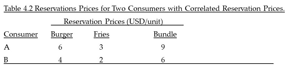
Bundling enhances profits only when consumers have uncorrelated reservation prices. In this way, bundling takes advantage of differences in consumer willingness to pay.
Many firms have used “Green Bundling” to tie goods with environmental or sustainable goods (natural, organic, local, etc.). As long as consumer preferences for the good and the sustainability goal are uncorrelated, this strategy will increase profits.
4.6.2 Tying
A practice related to bundling is tying.
Tying = The practice of requiring a customer to purchase one good in order to purchase another.
Tying is a specific form of bundling. An example is Microsoft selling Windows software together with Internet Explorer, a web browser. A second example is printers and ink cartridges. Many hardware companies make a great deal of profit from selling ink cartridges for printers. The cartridges do not have a universal shape, so must be purchased specifically for each printer. The next section will discuss advertising.
4.7 Advertising
Advertising is a huge industry, with billions spent every year on marketing products. Are these enormous expenditures worth it? The benefits of increased sales and revenues must be at least as large as the increased costs to make it a good investment. In this section, the profit-maximizing level of advertising will be identified and evaluated.
One important point about advertising is the costs associated with advertising expenditures. If advertising works, it increases sales of the product. There are two major costs, the direct costs of advertising and the additional costs associated with increasing production if the advertising is effective.
A typical analysis sets the marginal revenues of advertising equal to the marginal costs of advertising (MRA = MCA). This would be correct if the level of output remained constant. However, the output level will increase if advertising works, and the additional costs of increased output must be taken into account for a comprehensive and correct analysis, as will be shown below.
4.7.1 Graphical Analysis of Advertising
The graph for advertising is shown in Figure 4.11. Notice the two major effects of advertising and marketing efforts: (1) an increase in demand, in this case from D0 to DA, and (2) an increase in costs, shown here as the movement from ATC0 to ATCA. In the analysis shown here, advertising costs are considered to be fixed costs that do not vary with the level of output. This is true for a billboard, or television commercial. Note that the marginal costs do not change, since marginal costs are variable costs. The analysis could be easily extended to include variable advertising costs.
Economic analysis of advertising and marketing is straightforward: continue to advertise as long as the benefits outweigh the costs. In Figure 4.11, the optimal level of advertising occurs at quantity QA and price PA. Profits with advertising are shown by the rectangle πA. If profits with advertising are larger than profits without advertising (πA > π0), then advertising should be undertaken.
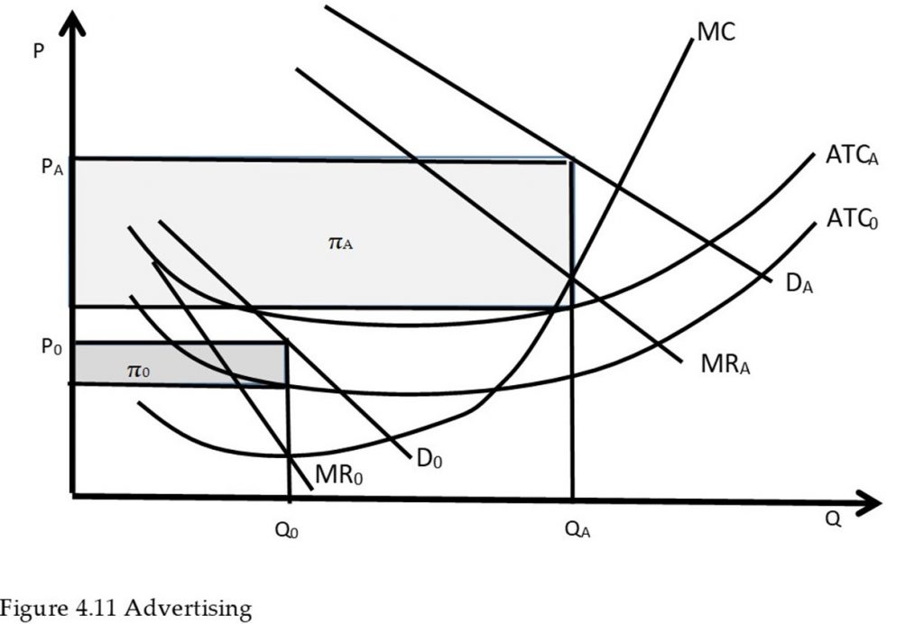
In general, if the increase in sales (DA – D0) is larger than the increase in costs, advertising should be undertaken. The optimal level of advertising can be found using marginal economic analysis, as described in the next section.
4.7.2 General Rule for Advertising
The profit-maximizing level of advertising can be derived, and the outcome is interesting and important, since it diverges from setting the marginal costs of advertising equal to the marginal revenues of advertising. Note that the graphical and mathematical analyses of advertising presented here could be used for any marketing program, not only advertising campaigns.
Assume that the demand for a product is given in Equation (4.4), where quantity demanded (Qd) is a function of price (P) and the level of advertising (A).
(4.4) Qd = Q(P, A)
This demand equation differs from the usual approach of using an inverse demand equation. For this model, it is more useful to use the actual demand equation instead of an inverse demand equation [P=P(Qd)]. The profit equation is shown in Equation (4.5), where the cost function is given by C(Q).
(4.5) max π = TR – TC
max π = PQ(P, A) – C(Q) – A
The profit-maximizing level of advertising (A*) is found by taking the first derivative of the profit function, and setting it equal to zero. This derivative is slightly more complex than usual, since the quantity that appears in the cost function depends on advertising, as shown in Equation 4.4. Therefore, to find the first derivative, we will need to use the chain rule from calculus, which is used to differentiate a composition of functions, such as the derivative of the function f(g(x)) shown in Equation (4.6).
(4.6) If f(g(x)) then ∂f/∂x = f’(g(x))*g’(x)
The chain rule simply says that to differentiate a composition of functions, first differentiate the outer layer, leaving the inner layer unchanged [the term f'(g(x))], then differentiate the inner layer [the term g'(x)].
In Equation (4.5), the cost function is a composition of the cost function and the demand function: C(Q(P, A)). So the derivative ∂C/∂A = C’(Q(A))*Q’(A) = (∂C/∂Q)*(∂Q/∂A). Thus, the first derivative of the profit equation with respect to advertising is given by:
∂π/∂A = P(∂Q/∂A) – (∂C/∂Q)*(∂Q/∂A) – 1 = 0
Rearranging, the first derivative can be written as in Equation (4.7):
(4.7) P(∂Q/∂A) = MC*(∂Q/∂A) + 1.
The term on the left hand side is marginal revenues of advertising (MRA), and the term on the right hand side is the marginal cost of advertising (MCA = 1), plus the additional costs associated with producing a larger output to meet the increased demand resulting from advertising [MC*(∂Q/∂A)].
This result can be used to find an optimal “rule of thumb” for advertising, or a “General Rule for Advertising.” There are three preliminary definitions that will be useful in deriving this important result. First, the advertising to sales ratio is given by A/PQ, and reflects the percentage of advertising in total revenues (price multiplied by quantity, PQ). Second, the advertising elasticity of demand is defined.
Advertising Elasticity of Demand (EA) = The percentage change in quantity demanded resulting from a one percent change in advertising expenditure.
(4.8) EA = %ΔQd/%ΔA = (∂Q/∂A)(A/Q).
Third, recall the Lerner Index (L), a measure of monopoly power. We derived the relationship between the Lerner Index and the price elasticity of demand, shown in Equation (4.9):
(4.9) L = (P – MC)/P = – 1/Ed.
With these three preliminary equations, we can derive a relatively simple and very useful general rule of advertising from the profit-maximizing condition for advertising, given in Equation (4.7).
P(∂Q/∂A) = MC*(∂Q/∂A) + 1
(P – MC)(∂Q/∂A) = 1
(P – MC)/P *(∂Q/∂A)(A/Q) = (A/PQ)
A/PQ = -EA/Ed
This simple rule states that the profit-maximizing advertising to sales ratio (A/PQ) is equal to minus the elasticity of advertising (EA) divided by the price elasticity of demand (–Ed). The result is simple and powerful: (1) if the elasticity of advertising is large, increase the advertising to sales ratio, and (2) if the price elasticity of demand is large, decrease the advertising to sale ratio. A firm with monopoly power, or a higher Lerner Index, will want to advertise more (Ed small), since the marginal profit from each additional dollar of advertising or marketing expenditure is greater.
Most business firms have at least crude approximations of the two elasticities needed to use this simple rule. Many firms advertise less than the optimal rate, since marketing can appear to be expensive if it is a large percentage of sales. However, simple economic principles can be used to determine the optimal, profit-maximizing level of advertising and/or marketing expenditures using this simple rule.
