6.1 Game Theory Introduction

Game theory was introduced in the previous chapter to better understand oligopoly. Recall the definition of game theory.

Game Theory = A framework to study strategic interactions between players, firms, or nations.

Game theory is the study of strategic interactions between players. The key to understanding strategic decision making is to understand your opponent’s point of view, and to deduce his or her likely responses to your actions.

A game is defined as:

Game = A situation in which firms make strategic decisions that take into account each other’s’ actions and responses.

A payoff is the outcome of a game that depends of the selected strategies of the players.

Payoff = The value associated with a possible outcome of a game.

Strategy = A rule or plan of action for playing a game.

An optimal strategy is one that provides the best payoff for a player in a game.

Optimal Strategy = A strategy that maximizes a player’s expected payoff.

Games are of two types: cooperative and noncooperative games.

Cooperative Game = A game in which participants can negotiate binding contracts that allow them to plan joint strategies.

Noncooperative Game = A game in which negotiation and enforcement of binding contracts are not possible.

In noncooperative games, individual players take actions, and the outcome of the game is described by the action taken by each player, along with the payoff that each player achieves. Cooperative games are different. The outcome of a cooperative game will be specified by which group of players become a cooperative group, and the joint action that the group takes. The groups of players are called, “coalitions.” Examples of noncooperative games include checkers, the prisoner’s dilemma, and most business situations where there is competition for a payoff. An example of a cooperative game is a joint venture of several companies who band together to form a group (collusioin).

The discussion of the prisoner’s dilemma led to one solution to games: the equilibrium in dominant strategies. There are several different strategies and solutions for games, including:

(1) Dominant strategy

(2) Nash equilibrium

(3) Maximin strategy (safety first, or secure strategy)

(4) Cooperative strategy (collusion).

6.1.1 Equilibrium in Dominant Strategies

The dominant strategy was introduced in the previous chapter.

Dominant Strategy = A strategy that results in the highest payoff to a player regardless of the opponent’s action.

Equilibrium in Dominant Strategies = An outcome of a game in which each firm is doing the best that it can regardless of what its competitor is doing

Recall the prisoner’s dilemma from Chapter Five.

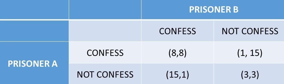
Figure 6.1 Prisoner’s Dilemma

 

6.1.2 Prisoner’s Dilemma: Dominant Strategy

(1) If B CONF, A should CONF (8 < 15)

(2) If B NOT, A should CONF (1 < 3)

…A has the same strategy (CONF) no matter what B does.

(3) If A CONF, B should CONF (8 < 15)

(4) If A NOT, B should CONF (1 < 3)

…B has the same strategy (CONF) no matter what A does.

Thus, the equilibrium in dominant strategies for this game is (CONF, CONF) = (8,8).

 

6.1.3 Nash Equilibrium

A second solution to games is a Nash Equilibrium.

Nash Equilibrium = A set of strategies in which each player has chosen its best strategy given the strategy of its rivals.

To solve for a Nash Equilibrium:

(1) Check each outcome of a game to see if any player wants to change strategies, given the strategy of its rival.

(a) If no player wants to change, the outcome is a Nash Equilibrium.

(b) If one or more player wants to change, the outcome is not a Nash Equilibrium.

A game may have zero, one, or more than one Nash Equilibria. The Prisoner’s Dilemma is shown in Figure 6.1. We will determine if this game has any Nash Equilibria.

 

6.1.4 Prisoner’s Dilemma: Nash Equilibrium

(1) Outcome = (CONF, CONF)

(a) Is CONF best for A given B CONF? Yes.

(b) Is CONF best for B given A CONF? Yes.

…(CONF, CONF) is a Nash Equilibrium.

(2) Outcome = (CONF, NOT)

(a) Is CONF best for A given B NOT? Yes.

(b) Is NOT best for B given A CONF? No.

…(CONF, NOT) is not a Nash Equilibrium.

(3) Outcome = (NOT, CONF)

(a) Is NOT best for A given B CONF? No.

(b) Is CONF best for B given A NOT? Yes.

…(NOT, CONF) is not a Nash Equilibrium.

(4) Outcome = (NOT, NOT)

(a) Is NOT best for A given B NOT? No.

(b) Is NOT best for B given A NOT? No.

…(NOT, NOT) is not a Nash Equilibrium.

Therefore, (CONF, CONF) is a Nash Equilibrium, and the only one Nash Equilibrium in the Prisoner’s Dilemma game. Note that in the Prisoner’s Dilemma game, the Equilibrium in Dominant Strategies is also a Nash Equilibrium.

 

6.1.5 Advertising Game

In this advertising game, two computer software firms (Microsoft and Apple) decide whether to advertise or not. The outcomes depend on their own selected strategy and the strategy of the rival firm, as shown in Figure 6.2.

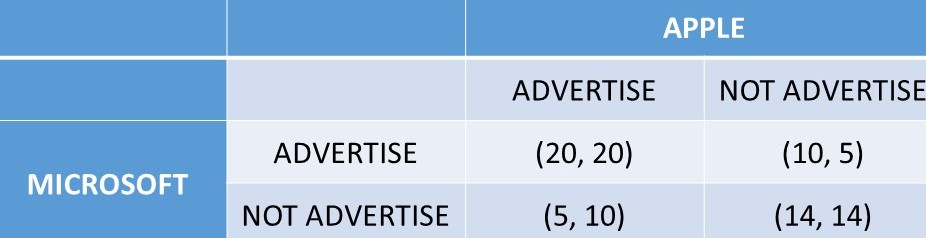
Figure 6.2 Advertising: Two Software Firms. Outcomes in million USD.

 

6.1.6 Advertising: Dominant Strategy

(1) If APP AD, MIC should AD (20 > 5)

(2) If APP NOT, MIC should NOT (14 > 10)

…different strategies, so no dominant strategy for Microsoft.

(3) If MIC AD, APP should AD (20 > 5)

(4) If MIC NOT, APP should NOT (14 > 10)

…different strategies, so no dominant strategy for Apple.

Thus, there are no dominant strategies, and no equilibrium in dominant strategies for this game.

 

6.1.7 Advertising: Nash Equilibria

(1) Outcome = (AD, AD)

(a) Is AD best for MIC given APP AD? Yes.

(b) Is AD best for APP given MIC AD? Yes.

…(AD, AD) is a Nash Equilibrium.

(2) Outcome = (AD, NOT)

(a) Is AD best for MIC given APP NOT? No.

(b) Is NOT best for APP given MIC AD? No.

…(AD, NOT) is not a Nash Equilibrium.

(3) Outcome = (NOT, AD)

(a) Is NOT best for MIC given APP AD? No.

(b) Is AD best for APP given MIC NOT? No.

…(NOT, AD) is not a Nash Equilibrium.

(4) Outcome = (NOT, NOT)

(a) Is NOT best for MIC given APP NOT? Yes.

(b) Is NOT best for APP given MIC NOT? Yes.

…(NOT, NOT) is a Nash Equilibrium.

There are two Nash Equilibria in the Advertising game: (AD, AD) and (NOT, NOT). Therefore, in the Advertising game, there are two Nash Equilibria, and no Equilibrium in Dominant Strategies.

It can be proven that in game theory, every Equilibrium in Dominant Strategies is a Nash Equilibrium. However, a Nash Equilibrium may or may not be an Equilibrium in Dominant Strategies.

 

6.1.8 Maximin Strategy (Safety First; Secure Strategy)

A strategy that allows players to avoid the largest losses is the Maximin Strategy.

Maximin Strategy = A strategy that maximizes the minimum payoff for one player.

The maximin, or safety first, strategy can be found by identifying the worst possible outcome for each strategy. Then, choose the strategy where the lowest payoff is the highest.

 

6.1.9 Prisoner’s Dilemma: Maximin Strategy (Safety First)

We use Figure 6.1 to find the Maximin Strategy for the Prisoner’s Dilemma.

(1) Player A

(a) If CONF, worst payoff = 8 years.

(b) If NOT, worst payoff = 15 years.

…A’s Maximin Strategy is CONF (8 < 15).

(2) Player B

(a) If CONF, worst payoff = 8 years.

(b) If NOT, worst payoff = 15 years.

…B’s Maximin Strategy is CONF (8 < 15).

Therefore, the Maximin Equilibrium for the Prisoner’s Dilemma is (CONF, CONF). This outcome is also an Equilibrium in Dominant Strategies, and a Nash Equilibrium.

 

6.1.10 Advertising Game: Maximin Strategy (Safety First)

(1) MICROSOFT

(a) If AD, worst payoff = 10.

(b) If NOT, worst payoff = 5.

…MICROSOFT’s Maximin Strategy is AD (5 < 10).

(2) APPLE

(a) If AD, worst payoff = 10.

(b) If NOT, worst payoff = 5.

…APPLE’s Maximin Strategy is AD (5 < 10).

Therefore, the Maximin Equilibrium in the Advertising game is (AD, AD). Recall that this outcome is one of two Nash Equilibria in the advertising game: (AD, AD) and (NOT, NOT). If both players choose Maximin, there is only one equilibrium: (AD, AD).

(1) The relationships between the game theory strategies can be summarized:

(2) An Equilibrium in Dominant Strategies is always a Maximin Equilibrium.

(3) A Maximin Equilibrium is NOT always an Equilibrium in Dominant Strategies.

(4) An Equilibrium in Dominant Strategies is always a Nash Equilibrium.A Nash Equilibrium is NOT always an Equilibrium in Dominant Strategies.

 

6.2 Cooperative Strategy (Collusion)

The cooperative strategy is defined as the best joint outcome for both players together.

Cooperative Strategy = A strategy that leads to the highest joint payoff for all players.

Thus, the cooperative strategy is identical to collusion, where players work together to achieve the best joint outcome. In the Prisoner’s Dilemma (Figure 6.1), the cooperative outcome is found by summing the two players’ outcomes together, and finding the outcome that has the smallest jail sentence for the prisoners together: (NOT, NOT) = (3, 3).

This outcome is the collusive solution, which provides the best outcome if the prisoners could make a joint decision and stick with it. Of course, there is always the temptation to cheat on the agreement, where each player does better for themselves, at the expense of the other prisoner.

Similarly, the cooperative outcome in the advertising game (Figure 6.2) is (AD, AD) = (20, 20). This outcome provides the highest profits (= 40 million USD) to both firms. Note that the advertising game is not a prisoner’s dilemma, since there is no incentive to cheat once the cooperative solution has been achieved.

 

6.2.1 Game Theory Example: Steak Pricing Game

A pricing game for steaks if shown in Figure 6.3. In this game, two beef processors, Tyson and JBS, are determining what price to charge for steaks. Suppose that these two firms are the major players in this steak market, and the outcomes depend on the strategies of both firms, since players choose which company to purchase from based on price. If both firms choose low prices, the outcome is low profits. Additional profits are earned by choosing high prices. However, when both firms have high prices, there is an incentive to undercut the other firm with a low price, to increase profits at the expense of the other firm.

Figure 6.3 Steak Pricing Game: Two Beef Firms. Outcomes in million USD.

 

6.2.2 Steak Pricing Game: Dominant Strategy

(1) If TYSON LOW, JBS should LOW (2 > 0)

(2) If TYSON HIGH, JBS should LOW (12 > 10)

…the dominant strategy for TYSON is LOW.

(3) If JBS LOW, TYSON should LOW (2 > 0)

(4) If JBS HIGH, TYSON should LOW (12 > 10)

… the dominant strategy for JBS is LOW.

The Equilibrium in Dominant Strategies for the Steak Pricing game is (LOW, LOW). This is an unexpected result, since it is a less desirable scenario than (HIGH, HIGH) for both firms. We have seen that an Equilibrium in Dominant Strategies is also a Nash Equilibrium and a Minimax Equilibrium. These results will be checked in what follows.

 

6.2.3 Steak Pricing Game: Nash Equilibrium

(1) Outcome = (LOW, LOW)

(a) Is LOW best for JBS given TYSON LOW? Yes.

(b) Is LOW best for TYSON given JBS LOW? Yes.

…(LOW, LOW) is a Nash Equilibrium.

(2) Outcome = (LOW, HIGH)

(a) Is LOW best for JBS given TYSON HIGH? Yes.

(b) Is HIGH best for TYSON given JBS LOW? No.

…(LOW, HIGH) is not a Nash Equilibrium.

(3) Outcome = (HIGH, LOW)

(a) Is HIGH best for JBS given TYSON LOW? No.

(b) Is LOW best for TYSON given JBS HIGH? Yes.

…(HIGH, LOW) is not a Nash Equilibrium.

(4) Outcome = (HIGH, HIGH)

(a) Is HIGH best for JBS given TYSON HIGH? No.

(b) Is HIGH best for TYSON given JBS HIGH? No.

…(HIGH, HIGH) is not a Nash Equilibrium.

Therefore, there is only one Nash Equilibrium in the Steak Pricing game: (LOW, LOW).

 

6.2.4 Steak Pricing Game: Maximin Equilibrium (Safety First)

(1) JBS

(a) If LOW, worst payoff = 2.

(b) If HIGH, worst payoff = 0.

…JBS’ Maximin Strategy is LOW (0 < 2).

(2) TYSON

(a) If LOW, worst payoff = 2.

(b) If HIGH, worst payoff = 0.

…TYSON’s Maximin Strategy is LOW (0 < 2).

The Maximin Equilibrium in the Steak Pricing game is (LOW, LOW). Interestingly, if both firms cooperated, they could achieve much higher profits.

 

6.2.5 Steak Pricing Game: Cooperative Equilibrium (Collusion)

Both JBS and Tyson can see that if they were to cooperate, either explicitly or implicitly, profits would increase significantly. The cooperative outcome is (HIGH, HIGH) = (10,10). This is the outcome with the highest combined profits. Both firms are better off in this outcome, but each firm has an incentive to cheat on the agreement to increase profits from 10 m USD to 12 m USD.