Appendix C. FFT Code Implementation
Appendix C. FFT Code Implementation
When programming the FFT in the C language, a couple “tricks” can make the process much more simple.
First, C does not have a “built in” complex data type, so an array of N complex numbers will actually be a 2*N floating point array. With the real and imaginary parts of the complex number in interleaved elements in the floating point array. The table below shows the way we access the various parts of the complex numbers that are represented by the floating point array.
| float f[2*N] | elements | “complex” C[N] |
| Index into f | Index into C | |
| 0 (2*0) | real part of C[0] | 0 |
| 1 (2*0+1) | imaginary part of C[0] | 0 |
| 2 (2*1) | real part of C[1] | 1 |
| 3 (2*1+1) | imaginary part of C[1] | 1 |
| 4 (2*2) | real part of C[2] | 2 |
| 5 (2*2+1) | imaginary part of C[2] | 2 |
| ... | ... |
In other words, real ( C[k] ) = f[2*k] and imag( C[k] ) = f[2*k+1].
Also, when we multiply two complex numbers, we have to work all the parts. As an example we will consider the case of two numbers, reC + j imC and cw + j sw. This is similar to what will be in the example c code, where
[latex]cw = cos( \frac{2 \pi}{N} ) " and " cs = sin( \frac{2 \pi}{N} )[/latex]
The product of these would look like
( reC + j imC ) * ( cw + j sw ) = ( reC * cw – imC * sw ) + j (reC * sw + imC * cw )
Finally it can be expensive to call cos and sin, thus we want to minimize these calls. So to step our basis function we will be using the following.
[latex]e^{-j \frac{2 \pi} {N} (k+1) } = e^{-j \frac{2 \pi} {N} k } * e^{-j \frac{2 \pi} {N} }[/latex]
Thus moving from k to k+1 only requires a single complex multiply. Also when we move from N length to N/2 length transforms we can avoid the function calls again by noting that
[latex](e^{-j \frac{2 \pi} {N} })^2 = e^{-j \frac{2 \pi} {N} 2 } = e^{-j \frac{2 \pi} {\frac{N}{2}} }[/latex]
Thus by squaring the term used in the previous stepping process, we would have the term needed for the next level of butterfly's. All of these "tricks" will come into play in the following code that implements the FFT.
This first set of code contains support functions that implement the butterflies used in the FFT, and does a bit reversal of the data, correcting for all the frequency decimation that occurs.
Figure 6.5 Code of Support Functions
Next is the code that will use the previous functions to implement the FFT. Note that an inverse FFT is done, by changing the terms cs and ss, to be the conjugates of the FFT implementation and including a loop to divide by 1/N.
Figure 6.6 Code Implementing the FFT and Inverse FFT.
Any software functions that are written should be tested at least to a basic functional level. For this purpose the following code, that calls the FFT and IFFT functions, was written and executed. The program generates a signal that has a cosine and a sine wave, which is done to demonstrate the response of the FFT to these fundamental coponents.
// Test array, Note it is twice as long fft (real and imaginary parts)
float x[2 * fft_len];
// Load array with test signal, having two simple components cos and sin
for (int i = 0; i < fft_len; i++)
{
x[2 * i] = (float)cos(pi / 2 * (double)i) + 0.5 * (float)sin(pi / 4 * (double)i);
x[2 * i + 1] = 0.0;
}
// Write input data to a file.
FILE* fout;
fopen_s(&fout, "Results.txt", "w");
for (int i = 0; i < fft_len; i++)
fprintf(fout, "%d, %f, %f \n", i, x[2 * i], x[2 * i + 1]);
// Perform FFT on test signal.
fft(x, fft_len);
// Write the transform to file.
fprintf(fout, "\n Input\n");
for (int i = 0; i < fft_len; i++)
fprintf(fout, "%d, %f, %f \n", i, x[2 * i], x[2 * i + 1]);
// Remove one of the components.
x[2 * 16] = 0.0;
x[2 * 16 + 1] = 0.0;
x[2 * 48] = 0.0; // Negative component removed
x[2 * 48 + 1] = 0.0; // to maintain symmetry.
// Perform inverse FFT.
ifft(x, fft_len);
// Write out output.
fprintf(fout, "\n Filtered Output\n");
for (int i = 0; i < fft_len; i++)
fprintf(fout, "%d, %f, %f \n", i, x[2 * i], x[2 * i + 1]);
fclose(fout);
// Exit
return 0;
Figure 6.7 Code Implementing the FFT and Inverse FFT.
The results from the program are include here as a table of results and later as a plot.
FFT of the input
0, 0.000000, 0.000000
1, 0.000000, 0.000000
2, 0.000000, 0.000000
3, 0.000000, 0.000000
4, 0.000000, 0.000000
5, 0.000000, 0.000000
6, 0.000000, 0.000000
7, 0.000000, 0.000000
8, 0.000000, 15.999994 // Component at pi over 4, purely imaginary for sine.
9, 0.000000, 0.000000
10, 0.000000, 0.000000
11, 0.000000, 0.000000
12, 0.000000, 0.000000
13, 0.000000, 0.000000
14, 0.000000, 0.000000
15, 0.000000, 0.000000
16, 32.000000, 0.000000 // Component at pi over 2, purely real for cosine.
17, 0.000000, 0.000000
18, 0.000000, 0.000000
19, 0.000000, 0.000000
20, 0.000000, 0.000000
21, 0.000000, 0.000000
22, 0.000000, 0.000000
23, 0.000000, 0.000000
24, -0.000002, -0.000002
25, 0.000000, 0.000000
26, 0.000000, 0.000000
27, 0.000000, 0.000000
28, 0.000000, 0.000000
29, 0.000000, 0.000000
30, 0.000000, 0.000000
31, 0.000000, 0.000000
32, 0.000000, 0.000000
33, 0.000000, 0.000000
34, 0.000000, 0.000000
35, 0.000000, 0.000000
36, 0.000000, 0.000000
37, 0.000000, 0.000000
38, 0.000000, 0.000000
39, 0.000000, 0.000000
40, -0.000001, 0.000000
41, 0.000000, 0.000000
42, 0.000000, 0.000000
43, 0.000000, 0.000000
44, 0.000000, 0.000000
45, 0.000000, 0.000000
46, 0.000000, 0.000000
47, 0.000000, 0.000000
48, 32.000000, 0.000000 // Component at -pi/2, purely real for cosine.
49, 0.000000, 0.000000
50, 0.000000, 0.000000
51, 0.000000, 0.000000
52, 0.000000, 0.000000
53, 0.000000, 0.000000
54, 0.000000, 0.000000
55, 0.000000, 0.000000
56, 0.000003, -15.999993 // Component at minus pi/4, purely imaginary for sine.
57, 0.000000, 0.000000
58, 0.000000, 0.000000
59, 0.000000, 0.000000
60, 0.000000, 0.000000
61, 0.000000, 0.000000
62, 0.000000, 0.000000
63, 0.000000, 0.000000
As noted in the printout of the results, the FT has distinct points that match up with the frequencies of the generated signal. The second part of the output from the program was a filtered version of the input. The numbers for the filtered signal can't be interpreted that easily, and would make more sense as a plot.
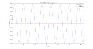
Figure C.1 Filtered Output Showing Only the Sine Wave at Pi/4.
The final test, although far from extensive, was intended to show that the FFT code was effective and functional.
